


 Inglés (pdf)
 Articulo en XML
 Referencias del artículo
 Enviar articulo por email
 Citado por SciELO
  Citado por Google
  Similares en
SciELO
Similares en
SciELO  Similares en Google
 Permalink
1. Introduction
The vehicle scheduling problem (VSP) is an optimization problem which is part of the operational planning of public transportation systems. In the VSP, tasks are assigned to buses to cover a given set of timetabled trips, considering different practical requirements and objectives. In this work, a real life vehicle scheduling problem is considered, derived from the operation of the mass transit system (MIO) in Cali city, Colombia. Some real constraints on the operation of some Colombian Bus Rapid Transit (BRT) systems, as well as the model proposed, are not found in previous models and literature reviewed. Before describing the problem, some definitions related to the problem addressed are mentioned, as well as the terminology used in the reviewed state of the art.
A trip is each one-way traversal of a route (line), characterized by: start location and time, end location and time. A task is a sequence of consecutive travels (trips) of a route between two stations. A block is one continuous chain of trips that start and end in depots. Two tasks T1 and T2 assigned to the same block are compatible if the start time of the second task is greater or equal to the time of completion of the first task plus the minimum time necessary to arrive the vehicle to the station where the second task begins. A deadhead trip is a trip without passengers (from a depot to a station or from a station to a depot). Two types of deadhead trips are named pull-out trip and pull-in trip. A pull-out trip corresponds to the movement of a bus from a depot to the start location of a trip, while a pull-in trip corresponds to the movement of a bus from an end location of a trip to a depot.
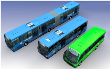
In the MIO system, four companies operate the system with four depots and three types of buses: Complementary (Compl), Articulated (Art) and Standard (Sta) [Figure 1].
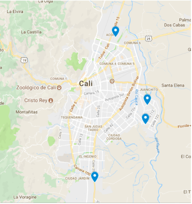
Each depot is administered by an operator and some of their locations are distributed in the city very distant from each other [Figure 2]. Then, the kilometers of a pull-in trip or pull-out trip can vary substantially, according to the depot assigned to these types of trips. Two kinds of tasks should be assigned to operators' buses: complete tasks (CT) or tasks in block (BT).
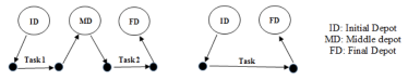
The planning period of each complete task is all day and a bus should service only one of these tasks; in the other case, a bus can serve one task (less frequent occurrence) or a block consisting of two tasks, which need to be compatible. All buses need to start and finish each task in a depot, not necessarily the same. Then, a CT is a sequence of the type: a pull-out trip, a task, and a pull-in trip. A BT is a sequence of the type: a pull-out trip, a task, two others deadhead trips (a pull-in trip and a pull-out trip, considering the same depot) a second task compatible with the first task and a pull-in trip [Figure 3].
Each type of vehicle can be assigned to both tasks. Two types of travel distances (in kilometers) are considered: commercial distances, associated to trips with passengers, and deadhead distances, associated to deadhead trips. The total commercial and deadhead distances should be distributed between the companies, according with the number of their buses assigned to the tasks. There are capacity constraints of depots, as well as a minimum number of parking spaces for buses of each operator in its own depot. The operators do not share buses. Each type of bus should be considered as a heterogeneous fleet, since only some of them are equipped with ramps to serve disabled people and some tasks, complete or not, require a bus to serve disabled people (called, to differentiate them from the rest, special buses).
Two main objectives are defined by the operators. One objective is to minimize the total deadhead kilometers. The other objective is to minimize the maximum deviation from the ideal amount of kilometers, both commercial and deadhead, determined using the share percentage of the operator’s buses in the system’s operation. The planning period is taken as a working day. The problem should be solved for each type of vehicle, but for each one of them differences should be considered, because by regulations of the mayor's office, some tasks at certain times must be assigned to special buses, named in this context special tasks. Then, a multi-vehicle-type model needs to be considered. Although there are routes with more demand than others, this is not taken into account in the model for the assignment of routes to the operators, as this aspect does not influence the profits they receive. In Section 3 it is explained why we do not include the minimization of the amount of used buses in the model.
We propose a mixed integer linear programming (MILP) formulation for this problem derived from the operation of the mass transit system in Cali city, Colombia. Nine representative instances were generated using real data obtained of the system operation. This paper is organized as follows. Section 2 presents the related work. Section 3 presents the proposed mathematical programming formulation. Section 4 reports numerical results obtained by running the proposed model on different representative instances, using real data of the operation of MIO system. Section 5 presents some variations to the proposed model. Finally, Section 6 concludes and gives some further research directions.
The main contribution of this paper is a model for a real VSP with some characteristics not considered in the literature, according to the review done. We used a realistic scenario for which improved solutions were found by applying the proposed model.
2. Related work
The vehicle scheduling problem (VSP) arises in public transport bus companies. In the VSP, tasks are assigned to buses to cover a given set of timetabled trips. There are some surveys of VSP, on the basis of a general problem definition [1-4]. A recent review of the literature on Transit Network Planning problems [5] includes the VSP, particularly the Multi-Depot VSP (MDVSP). Different approaches to model the VSP, solution methods and extensions for a better representation of real public transit systems, have been developed. Some of the extensions of the basic VSP consider MDVSP, heterogeneous fleet, and time constraints.
In MDVSP [6-19] vehicles are housed at the different depots, but each block of trips starts and ends at the same depot [10]. MDVSP are NP-hard [6]. Approaches to solve the problem based on a VSP with a single depot are in [7,8]. Mixed Integer Programming Problem formulations can be done based on trips [5,11-13] or less frequent, in blocks [8,14]. The MDVSP has been tackled in the literature by means of different approaches and formulations. Some representatives are: (a) a multi-commodity approach (6, 19), (b) a set-partitioning problem formulation using a column generation approach [15], and (c) a dynamic formulation [16]. One objective function proposed aims to minimize total deadhead kilometers, but if the fixed cost is adequately large, then aim of minimizing number of vehicles is prioritized [18]. A model and algorithm for the large-scale MDVSP was proposed [19] with departure-duration constraints based on the time-space network; the authors consider the practical factor that crews usually redefine shifts in the depot. There are different time constraints considered. For example, the total time a vehicle can be away from its depot is limited to a pre-specified time, taking into account real world operational constraints such as fuel consumption [9]. By including time windows in a VSP, it is allowed to shift scheduled trips within defined interval, in order to introduce flexibility in the departure times of trips [20]. Capacity constraints of depots are also considered [17].
Some papers about VSP include implementation of models and algorithms to real different VSP problems. A new approach for vehicle and crew scheduling, where the change of a vehicle of a driver is forbidden, is based on a maximum covering problem formulation and implemented with data of companies of Fortaleza, in Brazil [21]. In [11] is proposed a time window implementation to the multi-depot vehicle scheduling problem using a time-space network, testing the model on real-life timetables of some public transport companies of Germany. Based on this approach, a methodology was developed to implement time windows to the vehicle-type scheduling problem, and considering heterogeneous fleet [20]; the methodology was validated using real instances from a Brazilian city and large random instances. A comparative analysis of three vehicle scheduling models is made [10], including a multiple depot and two single depot vehicle scheduling models. This analysis is performed by solving the blocking problem for the operation of the Mass Transit Administration in Baltimore city, Maryland. Results obtained from the three models are compared with each other and the original schedule. The authors conclude that, under certain conditions, a single depot vehicle scheduling model performs better. Two types of disruptions arising in the MDVSP were considered: the delays and the extra trips [22]; these disruptions may or may not occur during operations, and they are indirectly incorporated into the planned schedule by anticipating their likely occurrence times. The objective functions more frequently used in a MDVSP are to minimize the total number of vehicles used, the total deadhead time (cost) of the operation, the operation time of the vehicles and a combination of some previous objectives. A simple model is proposed to assign 32 services to two operators of mass transit system (Megabús) in Pereira city, Colombia, through Goal Programming [23]; the objectives are: to minimize deadline kilometers, vehicle operating times, and discontinuous service. In the above paper, percentage of commercial kilometers assigned to operators is mentioned to be taken into account in constraints, but they do not appear explicitly in the proposed model, neither the other constraints. Simpler models of this case study, with capacity restrictions of depots discriminated by operator and minimizing deadline kilometers or net income, were presented in [24].
3. Proposed mathematical formulation
The following considerations are made:
As a result of a previous study of the data, regarding possible tasks to perform in blocks and their start and end times, two well-defined clusters of BT were obtained. The first (respectively second) cluster includes BT which can be assigned only as the first (respectively second) task in a block.
The previous pre-processing of tasks determines the number of total buses available in the model, so the total number of buses required is not minimized.
Each depot is represented by three dummy depots: an initial depot, a medium depot and a final depot. Then, each bus assigned to a block is associated with an initial depot, a medium depot and a final depot. These depots may be different or not, considering the real depots.
A weighted sum approach for this multiobjective problem is used. The first two objectives minimize the maximum deviation of kilometers (commercial and deadhead) assigned to the operators in relation to the ideal they should have according to the percentage of their buses in the fleet. The range of maximum deviation in commercial kilometers and deadhead kilometers are generally very different. These objectives produce min-max functions which need to be linearized. The third objective minimizes the total deadhead distance of the operation.
3.1 Notation and Modelling
Indexes
i: Tasks
k: Buses
j, r: Locations of depots, start points or final points of tasks
c: Operators
Sets
TP1: BT in the first cluster
TP2: BT in the second cluster
TP = TP1( TP2
CT: Complete tasks
PI: Initial Depots
PM: Middle Depots
PF: Final Depots
L: Locations of (TP ( PM)
B: Available buses
C: Operators
B(c) (B: Buses of operator c ( C
Parameters:
PP c : Share percentage of the operator c according to their available buses ((B(c)(/(B(), 0< PP c <1
KCO i : Commercial kilometers of task i.
KVA ri : Deadhead kilometers between a depot r and the initial or end station of a task i.
BE k : 1 if the bus k is a special bus, 0 otherwise
TE i : 1 if the task i requires a special bus, 0 otherwise
ESP c : Number of special buses of operator c
CAP r : capacity of depot r (number of buses)
PB c : Minimum number of buses of operator c that start or end tasks in its depot
T i : Departure time of task i
t jr : Average travel time from location j to r.
M: Upper bound, to condition values of variables in some constraints.
Decision variables:
x1irk: 1 if the task i ( TP1 is assigned to bus k ϵ B starting at depot r ( PI or ending at depot r ( PM(PF, 0 otherwise.
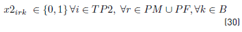
x2irk: 1 if the task i ( TP2 is assigned to bus k ϵ B starting at depot r ( PI(PM or ending at depot r ( PF , 0 otherwise.
xcirk: 1 if i ( CT is assigned to bus k ( B, starting at depot r ( PI, or ending at depot r ( PF, 0 otherwise.
s rk : Time in which bus k ( B arrives to r(L. (L is defined as Locations of (TP (PM)).
KC c : Commercial kilometers assigned to c(C
KV c : Deadhead kilometers assigned to c(C
desvkmc, desvkmv: Maximum deviation of commercial kilometers (desvkmc) and deadhead kilometers (desvkmv) which were assigned to operators in relation to the ideal quantity they should have.
α1, α 2, α 3: Weighting factors
3.2 Mathematical programming formulation
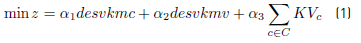
The mathematical model proposed is given in (1)-(33)
subject to:


In [1], α 1, α 2 and (3 include the weight given by the DM and the normalization schema in the weighted sum approach adopted.
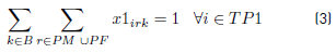
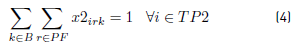
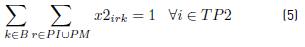
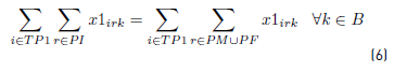
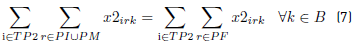
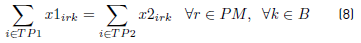
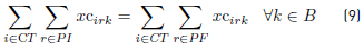
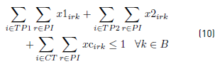
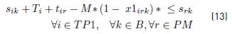
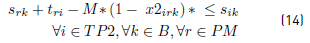
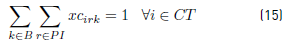
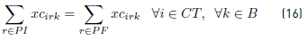
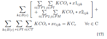
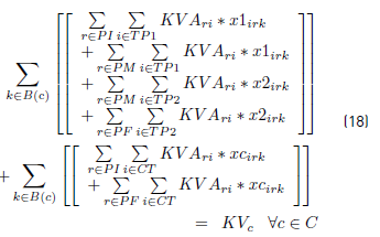
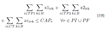
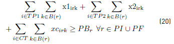
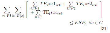
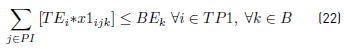
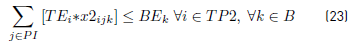
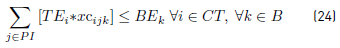
Constraints [2] to [5] ensure that to each task belonging to a block, a bus is assigned, and starts and ends exactly in a depot. Constraints [6] ensure that each bus assigned to a task on TP1 starts in a PI depot and ends in a PI or PM depot. Similarly, in constraints [7], each bus assigned to a task in TP2 starts in a PI or PM depot and ends in a PF depot. Constraints [8] ensure that any bus that arrives at a PM depot when finishes a task of type TP1, leaves this depot to start a task of type TP2. Constraints [9] ensure that each bus assigned to a task in CT begins in a depot (PI) and finishes in a depot (PF). In [10] each bus at most does a task of type TP1, TP2 or CT starting in a PI depot. Constraints [11] to [14] guarantee that two tasks assigned to the same block are compatible. Constraints [15] guarantee that each task in CT is done by a bus that starts in a PI depot. In constraints [16], it is ensured that each task in CT that starts in a PI depot, ends in a PF depot. In constraints [17] and [18] variables KCc and KVc represent the total commercial and deadhead kilometers, respectively, assigned to each operator c. They are really redundant, but make the model easier to understand. Constraints [ 19] ensure capacity constraints for each initial and final depot, while constraints [20] ensure minimum number of buses of each operator starting or ending tasks in its own depot. As each depot is administered by an operator, in constraints [20] B(r) means the set of buses in B(c), where c is the operator who administers the depot r. Constraints (21) ensure that no more special buses of each operator are used to do tasks requiring this type of buses, than the maximum available. Constraints [22] to [24] guarantee that a task that requires a special bus, is performed by a bus with these characteristics. [34] and [35] are the first two terms of the objective function, according to the operators’ objectives:
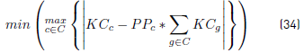
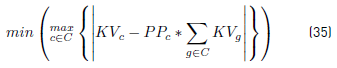
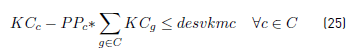
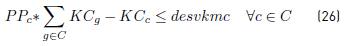
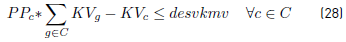
In order to obtain a linear model, the objectives given in [34] and [35] are obtained introducing the variables desvkmc, desvkmv and constraints [25] to [28]. Constraints [29] to [33] are domain constraints.
In a weighted sum approach, the weighting factors are generally composed by two factors: the weight given by the Decision Makers (DM) and a normalization factor. There are different possible normalization schemas, some of them are ineffective and not practical [25]. In this paper, the normalization and the weighting in the weighted sum approach are justified and contextualized to the case study presented, in Section 4.
In the literature reviewed, some requirements and objectives derived from the MIO operation in relation with buses, operators and depots are not considered: (a) special buses and special tasks as referred to in Section 1, (b) capacity restrictions of depots discriminated by operator and (c) the total assignment of buses to tasks per operator must be near to an ideal amount that depends on the operator’s share. The last two mentioned aspects not found in the literature have an important impact both on the values of the objective functions in the optimal solutions and in the execution times. It is shown in Section 4.
4. Validation of the proposed model
All tests were performed on an Intel Core i5-3210M 2.50GHz and 4 GB RAM. GUROBI was used for computing the solutions. Nine representative instances were generated from real data obtained from the operation of MIO System, and derived for the three types of buses, and three types of days: Working Day, any day between Monday and Friday (WD); Saturday (Sa) and Sunday (Su). Table 1 identifies each instance with the type of bus and type of day. In these types of days, the number of tasks and buses varies, in correspondence with the existent demand.
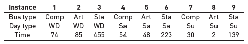
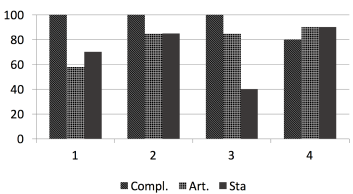
The operation of the system is considered in a representative month of the year and the data for each instance include: Minimum percentage of parking spaces for buses of each operator in its own depot [Figure 4].
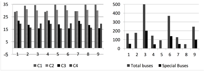
Buses per operator [Figure 5 Left, in percentage), also divided into special buses or not. Figure 5 (Right) shows total number of buses and special buses.
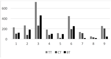
Complete tasks and tasks in blocks [Figure 6]. Tasks are also divided into special and not special tasks.
The normalization approach used is a variation of the method described in [25] using the ideal solution (z ideal ) and Nadir (z nadir ). Given the above values, each function f (x) is represented on a scale between zero and one, using the function (36)

In our model the z 𝑛𝑎𝑑𝑖𝑟 value for each function f i is the objective value offered by the current solution. The weighting factors in the objective function, taking into account the system managers, are: w1=w2=1, w3=0.5, because the profit per commercial kilometers made by each operator is more important than the cost of deadhead kilometers assigned to each one.
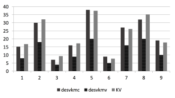
In all instances, the obtained solutions outperform the current solutions, taking into account the three objective functions. Figure 7 shows the percentage improvement of the solutions obtained with the application of the model.
The solutions are influenced by several factors: number of tasks to be assigned to buses, percentage of tasks in blocks in relation to complete tasks, number of tasks that must be taken into account for special buses, percentage of buses per operator and the minimum percentage of parking spaces for his buses in its own depot. The largest, and more difficult instance to solve, corresponds to working day and standard buses. The execution time (in minutes) ranged from 2 to 455. The execution times (in minutes) range from 2 to 455 and they are shown in Table 1. Its growth is not linear in function of the quantities of the different types of data (buses, tasks, etc.). Instance 8 was the easiest to solve. This instance does not consider special tasks, the proportion of BT tasks is less than CT tasks and it has the lowest total number of tasks to assign. Conversely, instance 3 was the most difficult, where the quantity of all types of data is the highest.
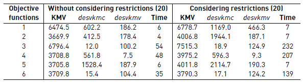
Two main aspects that make the solution of the problem most complex are: to consider the imbalance in the share of deadhead and commercial kilometers traveled by each one of the system operators and the constraint of a minimum number of buses of each operator starting or ending tasks in its own depot. To reflect the influence they have on the solution of the problem, and that differentiates this case study from other MDVSP seen in the literature, one of the instances was selected, considering the following objective functions:
O.F. 1: to minimize number of buses
O.F. 2: to minimize KV (total deadhead kilometers)
O.F. 3: to minimize desvkmc
O.F. 4: to minimize desvkmv
O.F. 5: to minimize the number of buses and deadhead kilometers (with the same normalization approach proposed and equal weight for both functions)
O.F. 6: to minimize (1desvkmc + (2KV
The first objective function is added since it is a usual objective for problems of type MDVSP. In our model, it is equivalent to maximizing the total number of blocks made where each block consists of two tasks, and the total of blocks is equal to the sum of the variables x1 irk , for i in TP1, r in PM, k in B. With each of the functions, two runs were made, one considering the restrictions [20] and the other eliminating them.
The obtained results are reflected in Table 2. The time is given in minutes. The number of buses used is not reflected in the table; with the objective functions 1 and 5 are equal and 5% less than with the other functions. As seen in Table 2, all results are deteriorated when the restrictions [20] are imposed. The execution times are significantly increased when the function to optimize consider the variables desvkmv and/or desvkmc. These conclusions are valid in the runs made with all the instances.
The results show the convenience of the development of heuristics in the solution of large problems when considering the first two objective functions of our model and the constraints [20].
5. Extensions to the proposed model
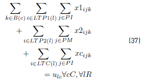
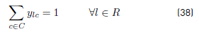
Some variations were developed to the proposed model. One of them was the addition of a new constraint, desirable (not mandatory) for the company: each route should be operated by the same operator. The model was modified in the following form:
New parameters:
M1: Upper bound (may be number total of tasks).
New sets:
R: Routes
LTP1(l): Tasks in TP1 of route l(R, LTP1(l) ( TP1
LTP2(l): Tasks in TP2 of route l(R, LTP2(l) ( TP2
LTC(l): Tasks in TC of route l(R, LTC(l) ( TC
New variables:
u lc : Number of tasks of route l assigned to some bus of operator c ϵ C.
y lc : 1 if at least a task of route l is assigned to some bus of operator c ϵ C.


Experimental results, with this new situation and the same instances described, show that there are not feasible solutions, due to the problem data. This result justifies incorporating this type of constraints as soft-constraints.
6. Conclusions and continuity proposals of this work
In this study, a new mathematical model is proposed to solve a multi-vehicle scheduling problem, derived from the operation of the mass transport system in the city of Cali, Colombia, which presents some characteristics not contemplated in the MDVSP type problems studied in literature and that make their solution more complex. The model was successfully solved, with nine representative instances generated with real data obtained from the operation of the system. However, only reasonable calculation times were obtained for the smallest instances in terms of all their parameters (tasks, buses, special tasks, tasks in blocks).
For future work, we identify the following four research lines: (a) proposing other methods to solve this multiobjective optimization problem, without considering the weighted sum approach; (b) adding other soft constraints suggested by operators, for example, to maximize the number of routes that a single operator must operate; (c) considering blocks with more than two tasks, and (d) proposing some heuristics in order to reduce the computational times, because the size of the problems may be increased in the near future and also it could be necessary to solve the problems with very short computational times; in certain situations, very efficient and fast heuristics will be necessary, as when a planned solution should be reoptimized in an operational context.

