


 Inglês (pdf)
 Artigo em XML
 Referências do artigo
 Enviar este artigo por email
 Citado por SciELO
  Citado por Google
  Similares em
SciELO
Similares em
SciELO  Similares em Google
 Permalink
1. Introduction
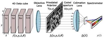
The acquisition of spectral images allows obtaining information from different ranges of the electromagnetic spectrum of a scene. The information can be represented as a data cube composed of different images at a specific wavelength, where each spectral band, provides information about the physical properties and distributions of materials in the scene [1]. On the other hand, one of the physical quantities associated with nature is polarization [2]. It measures information about the vector nature of the optical field in the scene, which allows knowing properties of the object surface such as roughness, shape, shading and orientation [3,4].
Spectral polarization images arise from the union of these two types of images, spectral and polarized, thus obtaining more information of the scene. Therefore, they have been used in diverse applications such as classification of vegetation [3], identification of surfaces contaminated with chemical agents [5], and biomedical diagnosis in the analysis of skin [6]. The major difficulty with spectral polarization images is their acquisition, because it needs to sense the spatial, spectral and polarization information,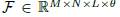 (see Figure 1]. For instance, an image with M = N = 256, L = 14 and θ = 4 demands sensing and storing more than 3 million voxels. Traditional acquisition methods use a linear polarizer that is rotated while sequential measurements are captured, spanning the scene in each dimension [7] or by changing the set of color filters [8]. The time required for these methods depends directly on the speed of change of these optical elements, therefore limiting their usage in dynamic sensing while the noise increases due to the changing mechanisms.
On the other hand, compressive sensing devices used in spectral polarization imaging obtain compressed projections of a scene, where the number of samples is smaller than the total amount of scene voxels, which enable faster acquisitions. For instance, recent works have shown good results with as few as 20% of compressed measurements [9-11] which would reduce by 80% the acquisition time of traditional methods. The techniques of compressive sensing imaging (CSI) are able to reconstruct the image from an underdetermined system of linear equation that describes the measurement acquisition process [12,13], by choosing an appropriate representation basis where the image presents sparse behavior [14].
A single-pixel polarimetric imaging spectrometer was proposed recently, enabling the acquisition of spatial, spectral, and polarization information about the scene from compressive measurements [10]. This architecture utilizes a Digital Micromirror Device (DMD) as a spatial light modulator. The spectral polarization analysis is achieved by combining a rotating polarizer with the spectrometer. However, compression occurs in the spatial domain, while spectral and polarization dimensions are preserved. Consequently, hundreds of sequential measurements are needed to obtain a good construction.
Another compressive spectral polarization imaging technique that uses a pixelized polarizer and colored patterned detector (CSPI) was proposed in [9], this architecture employs a pixelized polarizer and colored patterned detector that enables compressive sensing over spatial, spectral, and polarization domains. However, this architecture only allows four different acquisitions of the scene and its associated cost increases as either more filters are added to the detector or the sensor resolution increases. This limits the use of this system. Therefore, achieving a high quality reconstruction with a low-resolution camera is desired.
For this reason, this paper proposes an alternative to reduce the acquisition cost of the spectral polarization images, since it uses a single pixel as the detector. In addition, this architecture can capture multiple shots, using a movable pixelized polarizer and the binary coded aperture. In this way, obtaining spectral and polarization information of the scene from few compressed spatial-spectral and polarization information measurements.
2. Spectral Polarization Images
Spectral polarization images can be modeled as a 4D structure, shown in Figure 1, where each 3D image represents the scene at one of the four polarization angles (0°, 45°, 90°, 135°). This representation does not modify the spatial structure of the scene. One of the most common ways to represent polarization is by means of the Stokes parameters S. These are four vectors that describe partial or total polarization of light based on intensity measurements [15]. Stokes vectors are defined in terms of optical intensity as follows: S 0 is the total intensity of a scene, S 1 is the difference between the intensity along the x (0°) axis, and the one oriented parallel to the y (90°) axis, S 2 is the difference between the linear +45° and -45◦ polarization and S 3 is the difference between the intensity transmitted by a right circular polarizer and a left circular polarizer [16]. In the majority of applications, the S 3 component is not used; additionally, sensing S 3 requires an additional quarter-wave plate [17], which is not considered in this work. For this reason, it is typical to work with only the first three Stokes vectors, which have a linear relationship with the measurements of the traditional detectors. These are given in Equations (1), (2) and (3) as follows


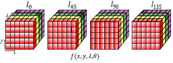
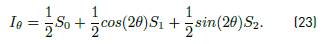
where I θ is the polarization intensity at the angle θ, S 0 is the total radiation of a beam, and S 1 and S 2 are the radiation difference of the linearly polarized beam, these parameters are visualized in Figure 2.
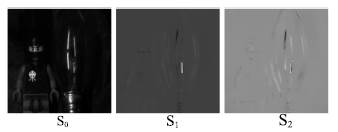
Figure 2 Visual representation of the Stokes parameters in black and white images. a) S 0, b) S 1 and c) S 2 at a wavelength of 530 nm
The angle of polarization (AoP), which is defined by Equation (4), specifies the orientation of the beam oscillation [9], which in terms of the Stokes parameters can be represented by
As we can see, the angle depends only on the parameters S 1 and S 2.
3. Sampling Process
To capture spectral polarization images in a compressed manner, we propose the optical architecture shown in Figure 3. There, the scene is encoded in polarization and in spectrum by the pixelated polarizer and the coded aperture. Then the coded scene passes through the condenser lens, which concentrates the light to a point, creating a mixed pixel, which contains all the encoded information. This point is integrated by the spectrometer that divides the information into spectral ranges.
In the sampling scheme, the scene is represented by  where x and y represent the two spatial dimensions, λ is the spectral wavelength, and θ represents the angle of linear polarization. By considering the possibility of applying multiple measurements, the scene passes through a polarization filter array
 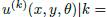 1,…,K, that allows or not the pass of a certain polarization angle per pixel, with K possible patterns. Then it encounters a coded aperture
  = 1,…,K, which applies spatial modulations to the scene. Ideally, u and c are binary functions, the blocks blocking or not the passing of voxels in the 4D data cube. In this way, the spatial, spectral and polarization modulated scene is obtained as in Equation (5)

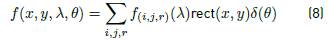
Let 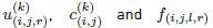 be the discretized polarization filter array, the discretized coded aperture and the discretized data respectively defined in Equation (6), (7) and (8) as
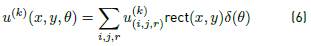
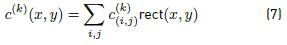
Where
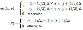
are the 2D and 1D sampling functions respectively, Δ is the sample pixel size which is assumed equal for the micro-polarizer array, the coded aperture and the images and Δ θ is the sample angle. The discrete form describing the modulation of the scene given in Equation (5) is expressed in (9) as:
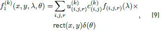
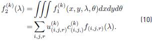
and the continuous model for the spectral density through the coded aperture, the polarization filter array and the optics before it impinges the sensor array is given by Equation (10)
In the proposed sensing model, the scene is viewed as four linear polarization intensity cubes indexed by r = 1; 2; 3 and 4 indicating cubes with four polarization angles and Δ
θ
= 45. Also, the spectral range of the instrument is partitioned into a finite number of subintervals or channels. The discretization of the spectral axis is given as λ
(l)
for l = 1, …, L where L is the number of spectral bands. The range of the channel l is  where λ
(l)
is the solution of the Equation (11)
where λ
(l)
is the solution of the Equation (11)

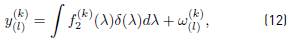
where this pixel is taken by the spectrometer to obtain measurements by spectral bands in (12) as
Where
 is additive noise in the sensor and Δ
λ(l)
= λ
(l+1)
- λ
(l)
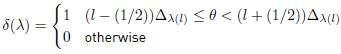
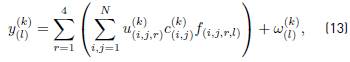
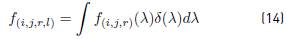
; l = 1 ,…, L is the range of the spectral band l. Finally, in Equation (13) and (14) the discrete model to obtain the measurements is given as
is additive noise in the sensor and Δ
λ(l)
= λ
(l+1)
- λ
(l)
; l = 1 ,…, L is the range of the spectral band l. Finally, in Equation (13) and (14) the discrete model to obtain the measurements is given as
With
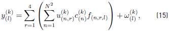
is the discretized data and N is the spatial resolution. By converting from row-column subscripts into linear indexing as n = N(i - 1) + j, for i; j = 1 ,…, N, the Equation (13) becomes (15) as
and the matrix form is expressed in Equation (16) as
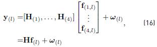
where 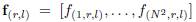 is the vectorization of the spectral polarization imaging in the angle r and band l,
  are the compressive measurements in the band l and
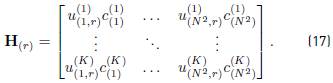
 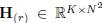 is the sampling matrix which is determined by the polarized and coded aperture in Equation (17) as
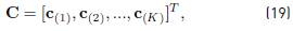
Because all spectral bands are encoded with the same coded aperture pattern, in Equation (18) the problem can be seen in a vector way as

where  are the compressive measurements obtained by the spectrometer in K shots,
 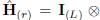 H
(r)
, where I
(L)
is an identity matrix of size L,
H
(r)
, where I
(L)
is an identity matrix of size L,  denoted the Kronecker product, and f
(r)
are the vector images at the angle r.
denoted the Kronecker product, and f
(r)
are the vector images at the angle r.
3.1 Measurement hardware strategy
The vector form of the coded aperture is given by c
(i)
= 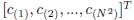 for k = 0; 1, …, K. Expressing the set of coded apertures and considering K total shots in Equation (19) we have
Where  represents the binary value (white translucent or block). Designing an array of polarizers that changes at each acquisition is expensive [9], this paper proposes designing one with dimensions
  , such that for each capture, the array of polarizers is moved horizontally in a pixel. Mathematically,U can been seen as a 3D array of binary elements that represent the pixelated polarizer, (see Figures 4(a) and 4(b)) in which an angle r is represented as
  where
where  for r = 1; 2; 3; 4. Then, in Equation (20) for each shot we have
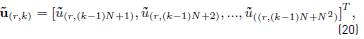
for k = 0, 1, …, K which represents the horizontal movement of a pixel for the angle r, this can be seen in Figure 4(c) for the first vector of  The binary matrix is expressed in Equation (21), which represents all the acquisitions

where 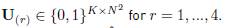
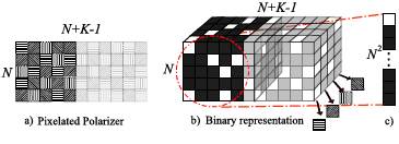
Figure 4 Representation of the pixelated polarizer a) visual representation b) binary representation c) vectorization of the first angle and first shot of the binary representation
The sampling matrix  which is determined using Equation (22) , represents the sampling, modulation and the different captures of the spectral polarization images. The information that this matrix has is shown in a specific order as:
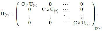
where  is the Hadamard product between the matrices C and U(r). A graphical representation of the sampling matrix is shown in Figure 5, For this example, an image with 4 x 4 pixels of spatial resolution, 3 spectral bands, 4 polarization angles and 50% of compression is used. The compression rate is calculated as
  . The white points represent the unblocking pixel (1), while the entries (0) are represented in black.
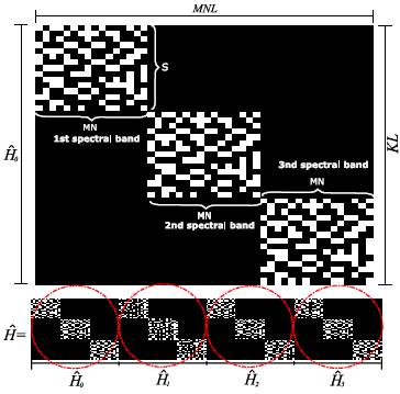
Figure 5 Illustrative example of the sensing matrix  for N = 4;M = 4;L = 3. White points have the values of 1 and black points are 0
The relationship between the intensity of the light passing through a θ° linear polarizer I θ and the Stokes parameters S 0 to S 2, of the original light, is linear and given by the following Equation (23)
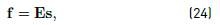
Therefore, the vectorized linear polarization cubes f have a linear transformation with the three first three Stokes parameter cubes s, as shown in Equation (24)
Where 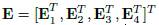 and
and 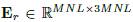 consist of three diagonal block matrices expressed in Equation (25) as:
for the four values of θ(r) with r = 1, …, 4. Thus, the sensing process referent to the Stokes parameter can be expressed, as in Equation (26)

where G represents the sensing process from the tree Stokes parameter cubes directly to the measurements. Due to matrix  having inputs 1 and 0, and E entries given in Equation 25, the values of G are given from the set
 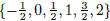 . In order to see the sensing matrix G an image of 4 x 4 pixels of spatial resolution, 3 spectral bands, 4 polarization angles and 50% of compression is used. The new compression rate with respect to Stokes parameters is calculated as
  , where 3 are representing the three first Stokes parameters. The blue points represent
  , black represents 0, green represents
  , white represents 1, red represents
  and finally yellow represents 2. In Figure 6 the sensing matrix can be seen, that represents the first parameter where its minimum value is 0 and its maximum value is 2, and for the other two parameters the values are
  due to the values taken by the product between and E.
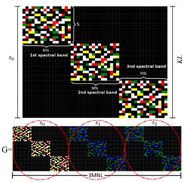
Figure 6 Illustrative example of G, which is composed of the three sensing matrices corresponding to the first three Stokes parameters for N = 4;M = 4;L = 3. Blue points represent black points are 0, green represents  , white points have the values of 1, red represents and yellow points are 2
To exploit the sparsity of the data cube, each Stokes parameter is represented by a three dimensional Kronecker basis 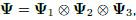 , where
  is the 2D-Wavelet basis that provides the basis in the spatial domain and
  is the discrete Cosine basis that is the basis in the spectral domain. In this case
  thus the sensing process can be expressed in Equation (27) as

where A is the composite sensing matrix that modules the system. The signal recovery is obtained by solving the inverse problem of the under determined linear system in (27). This consists in recovering Θ such that the l1 - l2 cost function is minimized [14,18]. The optimization problem is given Equation (28) as
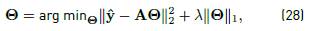
where λ is a regularization parameter. The Gradient Projection for Sparse Reconstruction (GPSR) algorithm [19] is used to solve Equation (28) in this work.
4. Design of the sampling matrix based on Hadamard matrices
Recent work has shown that designing sampling matrices significantly improves the quality of the reconstruction [20- 22]. In this section, the Hadamard matrix is used to design the sensing matrix since its rows are mutually orthogonal; this property is desired in compressive sensing [12,23]. This property allows a fast reconstruction approach, due to the transpose normally used in the GPSR algorithm is reduced to only one matrix product [18, 24]. Thus, Equation (29) is
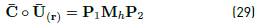
Where  is a Hadamard matrix,
 is an incomplete permutation matrix that only has a one-valued entry on each row and
  is a permutation matrix which operates over the columns of M
h
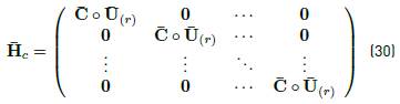
[25]. Therefore, the sensing matrix is now expressed in Equation (30) as
is a permutation matrix which operates over the columns of M
h
[25]. Therefore, the sensing matrix is now expressed in Equation (30) as
In order to apply this codification the entries of  should be {-1,1} instead of {0,1}. For this, the measurements y
0 = Df are firstly taken, where D is a sensing matrix with C
(i;j)
= 1 and U
(r;i;j)
=
should be {-1,1} instead of {0,1}. For this, the measurements y
0 = Df are firstly taken, where D is a sensing matrix with C
(i;j)
= 1 and U
(r;i;j)
=  , letting all the information of the scene pass in an acquisition. The codified measures obtained with {-1,1} for each shot are calculated using Equation (31) as
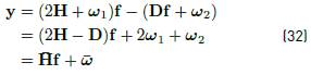

Where  represent a shot of the sensing matrix expressed in (30). The problem with noise is expressed in Equation (32) as
Where  is the noise present in the process. The sensing and reconstruction referring to the parameters of stokes are followed from Equation (26) replacing
  .
.
5. Simulations and Results
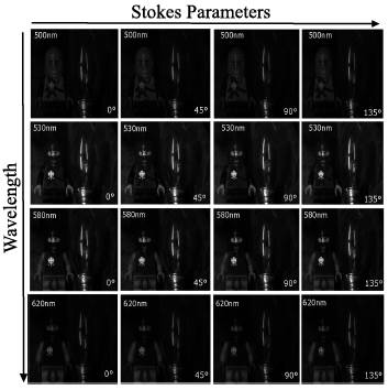
To evaluate performance and study the proposed compressive sensing system, simulations were performed with a 4D test data array, which contains four cubes of polarization intensities that were acquired by switching fourteen bandpass filters combined with four azimuth angles (0°, 45°, 90° and 135°) of a linear polarizer (LPVISB100-MP2). Each cube with polarization intensity contains fourteen (L = 14) spectral bands ranging from (500 nm to 620 nm), with spatial resolution of 256 by 256. The scene was illuminated with unpolarized light. In Figure 7 the scene shows the four polarization angles in four different spectral bands.
The linear polarization information is obtained by Eqs. 1, 2 y 3. Figure 8 shows the Stokes parameters for four different wavelength. The second and third Stokes parameters represent the linear polarization state. In the 4D array of data, a toy and a bulb can be seen, each with different textures and shapes. With this four-dimensional data cube, simulations can be performed using Equation. 15 without additional noise.
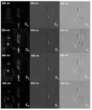
Figure 8 Stokes parameter S0, S1 and S2 for each data cube is shown in four of 14 bands of polarization: 500, 530, 580 and 620 nm
The proposed architecture was compared with CSPI [9], this was used with random inputs for the micropolarizer and the colored filter array. The GPSR algorithm was used to reconstruct the Stokes parameters from compressed measurements for both architectures. The peak signal-to-noise ratio (PSNR) is used to measure the quality of the reconstructed Stokes parameters.
The compression level of CSPI is given as  , where P = 3 is the number of Stokes parameters used, S is the number of shots and Nm = (M + L - 1)N is the number of measurements in a single acquisition. It should be clarified that, for this architecture only 4 shots can be made, because the prism is rotated only in 4 angles, so for a single shot its compression level is 2.5% and the maximum compression level for this architecture would be 10% for these images. On the other hand, the compression level of the proposed architecture is given as
  . In our architecture, the number of different captures depends on the size of the micro-polarizer and because there is a coded aperture that may vary with each shot, the number of encodings other than the scene for a single movement of the micro-polarizer is given by
  where
where 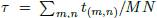 is the quantity of energy that passes through an object known as transmittance, allowing multiple acquisitions.
Figure 9 shows the average PSNR of 20 iterations for different levels of compression from 5% to 10% with step of 2,5 and from 10% to 50% with step of 5, for 3 stokes parameters reconstructed. It can be seen that, for 2:5% to 10% levels of compression the proposed architecture outperforms CSPI in the parameters S 1 and S 2. In a particular case, for 2:5% the proposed method overcomes up 4:5 dB and 5:3 dB for S 1 and S 2 respectively, for the parameter S0 both methods have a similar quality. The dotted line represents the maximum PSNR achieved by CSPI because taking more snapshots is not possible.
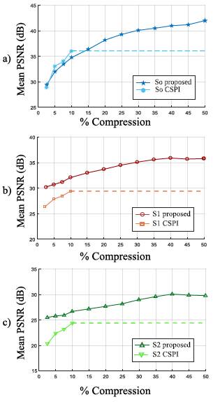
Figure 9 Mean PSNR of 20 iteration for different levels of compression from 5% to 10% with step of 2,5 and from 10% to 50% with step of 5, for a) the first b) the second and c) the third parameter reconstructed
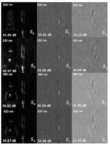
To visualize the reconstruction quality, the reconstructed Stokes images plane in four spectral channels for 10% of compression are displayed in Figure 10 for both architectures. The reconstruction shows significant image quality compared to CSPI.
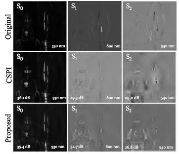
Figure 10 Reconstructed Stokes parameter S 0, S 1 and S 2 using the proposed and CSPI architecture. The parameter S 0 is displayed in the band 530 nm, S 1 in the band 600 nm and S 2 in 540 nm
In order to verify the spectral accuracy of the proposed architecture, three spectral points of the original data cube are compared with the reconstructed signatures. In Figure 11 the results are presented. In general, the results show that the proposed architecture presents better spectral performance than CSPI.
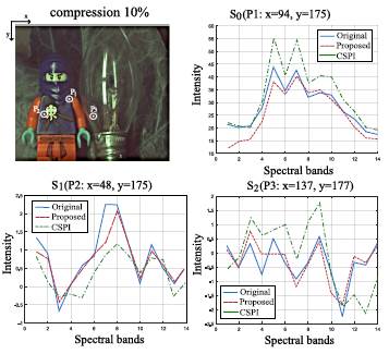
Figure 11 a) RGB image of the sample and spectral signatures obtained in the reconstructions with the proposed and CSPI architectures, in the points of the image b) P1 (x = 94, y = 175) in the parameter S 0 c) P2 (x = 48 , y = 175) in parameter S 1 and d) P3(x = 137, y = 177) in parameter S 2
Finally, to visualize the reconstruction quality with more level of compression Figure 12 shows reconstructed Stokes parameters for each data cube in four of 14 bands of polarization: 500, 530, 580 and 620 nm. It can be seen that with 30% of compression the reconstruction has good image quality.
6. Conclusion
The mathematical and matrix model for the single-pixel architecture for the compressive acquisition of spectral polarization images was developed. The architecture presented makes use of a micro-polarizer that allows or denies the propagation of the polarization angles of the image, a coded aperture that allows the spectral and spatial coding, the collimator modulates the information to a pixel and this is classified in spectral bands using the spectrometer. The coding of the scene produced by the micro-polarizer and the coded aperture was analyzed for different levels of compression, the results show a gain of up to 3dB for 10% compression in the parameters S1 and S2 compared to CSPI architecture, also, 30% compression exhibited stable quality for the studied image. Future work includes the implementation of the proposed architecture to validate the obtained results in a real scenario.

