1. Introduction

Wireless Sensor Networks (WSNs) are composed of sensor nodes with constrained resources. The nodes measure a physical variable (e.g., temperature, humidity, or light) in an area of interest, and then, send this information to the sink. WSNs do not rely on pre-existing infrastructure, so, the network topology is built by the nodes once deployed. Initially, the nodes do not have any previous knowledge about their neighborhood because they are scattered randomly, so, they collect information about their neighbors and the link quality using a procedure called neighbor discovery. Using this information, each node computes routes to reach the sink through multiple hops. In this paper, we propose an algorithm called Dynamic Gallager-Humblet-Spira (DGHS) that builds and maintains a minimum spanning tree which we use to collect data.

In WSNs, finding the optimal route from each node to the sink is not straightforward because of the distributed and dynamic features of the network. On the one hand, the nodes should avoid any centralized control that depletes their energy by sending control packets over long distances. Instead, they should collaborate among them through the exchange of local information. On the other hand, the network is dynamic because of the frequent changes: the channel quality varies over time, and the nodes can join or leave the network as a result of mobility or battery exhaustion [¹]. Thus, mechanisms for topology construction and maintenance must be distributed and adapt to the dynamic features of the network.

Depending on its internal rules, topology construction mechanisms can lead to different types of structures, such as trees, clusters, or meshes. In the tree topology, each node selects a single parent that receives and forwards the data packets. The parent selection determines how and when the tree is built, so, it is the core of the tree construction mechanisms. The criteria for selecting a neighbor as a parent is different for every application. When the parent selection is over, a tree topology rooted at the sink is available. This tree topology is suitable for WSNs since it enables the many-to-one communication needed to collect data.

Many mechanisms have been proposed to construct a tree topology (See Section 2). However, few mechanisms work in a distributed manner and adapt the tree to the dynamic features of the network. In this paper, we propose a distributed and dynamic algorithm called Dynamic Gallager-Humblet-Spira (DGHS) that builds and maintains a minimum spanning tree. DGHS is based on the Gallager-Humblet-Spira (GHS) [², ³] algorithm. Note the distinction between DGHS - our mechanism - and GHS - the algorithm proposed by Gallager Humblet Spira. GHS is a static algorithm that finds the minimum spanning tree in a network but does not repair the topology when node failures occur. Additionally, GHS is a theoretical work that has not been evaluated on a wireless network setting. Thus, the contributions of DGHS are twofold: First, DGHS extends GHS by repairing the tree when node failures occur; and secondly, to the best of our knowledge, this is the first paper that evaluates a GHS-based algorithm for a WSN.

DGHS has four phases, namely neighbor discovery, tree construction, data collection, and tree maintenance. In the neighbor discovery, the nodes collect information about their neighbors and the link quality. In DGHS, the link quality is defined as the average number of lost discovery packets. In the tree construction, DGHS finds the minimum spanning tree by executing GHS. In GHS, each node is a different fragment. Subsequently, pairs of fragments merge into a new one. The fragments continue to join until only one remains: the final fragment is the minimum spanning tree. This minimum spanning tree generated by GHS is not rooted at the sink. Thus, in the data collection phase, the sink roots the minimum spanning tree at itself by sending a single control message via the branches of the tree. Then, each node starts sending data packets. In the tree maintenance phase, the nodes repair the tree when communication failures occur (i.e., the nodes cannot communicate anymore) by merging disconnected fragments. The repair mechanism is initiated by the sink and partially reruns GHS to join disconnected fragments.

We implement DGHS on Contiki which is a widely used open-source operating system for low-power and memory-constrained devices. Subsequently, we evaluate the performance of DGHS on Cooja which is the Contiki network emulator. We compare DGHS with a state-oftheart tree construction mechanism known as Least Path Interference Beaconing Protocol (LIBP) [⁴, ⁵]. The results show that DGHS uses fewer control packets and consumes on average less energy than LIBP, at the cost of a slight increase in the memory size and convergence time.

Specifically, the results show that DGHS uses 25.6% fewer control packets than LIBP during the tree construction. Besides, DGHS consumes on average less energy that LIBP: it consumes on average 0.6mW less during the tree construction, and 1.9mW less during the data collection. These results are explained given that DGHS is messageoptimal and sends the data packets through the optimal route (i.e., via the minimum spanning tree). Moreover, DGHS shows a slightly higher memory consumption and slower convergence time because of its complexity.

When compared to our previous work [⁶], this paper presents: (i) a detailed description of the stages of the DGHS algorithm (neighbor discovery, tree construction and data collection), (ii) an in-depth analysis of extensive results that validates our proposal, and (iii) an exhaustive description of the limitations of GHS for WSNs.

This paper is organized as follows: Section 2 presents recent work about tree construction mechanisms; Section 3 briefly describes GHS and its limitations; Section 4 explains in detail the DGHS algorithm; Section 5 shows the evaluation setting and the performance metrics; Section 6 evaluates the performance of DGHS and LIBP; and, Section 7 presents our conclusions and future work.

2. Related work

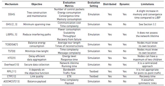
The problem of constructing and maintaining a tree topology in a distributed manner is a challenging task. This is because the nodes have limited computational and memory resources and the network is dynamic: the nodes are prone to failures, and the channel quality varies over time [¹]. We present relevant work that aims at solving this problem and summarize our findings in Table 1. Note that this table also serves as a qualitative comparison of DGHS with previous work.

Table 1 Previous work regarding tree construction mechanisms 

In [⁴, ⁵], the authors present a protocol called Least Path Interference Beaconing (LIBP) that constructs a tree which reduces the interference on the parent nodes. To do that, LIBP limits the number of children that each parent supports. The tree construction is done by sending periodic beacons. Initially, the sink broadcasts a beacon including its identity and weight. Upon reception of this beacon, the nodes reply with an acknowledgment (ACK) informing the sink that it has new children. Then, the sink increments its weight according to the number of new children. By repeating this process, LIBP creates a tree topology that reduces the interference on the parent nodes. Moreover, LIBP repairs the network in the event of parent failure.

[⁷] presents in-depth an algorithm called TCBDGA (Tree-Cluster-Based Data-Gathering Algorithm). It constructs several tree topologies that gather data using a mobile sink. Initially, the nodes build a single tree topology by selecting a parent according to the residual energy, the distance to the sink, and the local node density. Subsequently, this tree is decomposed into sub-trees considering its depth and traffic load. Finally, the mobile sink visits the sub-trees to collect data and to reconstruct them when their residual energy is low. In [⁸], the authors present an algorithm called Toward Source Tree (TST) that constructs a tree which forwards information from a source to multiple receivers (i.e., a multicast tree). TST aims at minimizing the tree length and, as a consequence, the delay. To do that, a virtual tree is built by using only the receivers. Subsequently, pairs of receivers are connected by finding relay nodes between them. Finally, the possible cycles are eliminated from the resultant tree. The drawback of TST is that it assumes that the nodes know their location and it does not work for dynamic networks.

[⁹] presents an algorithm called Hybrid Tree Construction (HTC) that builds and maintains a tree in which the nodes can only have two children (i.e., a binary tree). By using this tree structure and a time slot scheduling, the nodes aggregate data. The tree construction starts with a neighbor discovery that assesses the energy level and response time of the neighbors. Subsequently, each node selects a parent and a child based on the lowest response time guaranteeing a minimum delay. If two neighbors have the same response time, then the energy level is used as a tiebreaker. Moreover, HTC re-constructs the tree in case of nodes failure.

In [¹⁰], the authors construct a shortest-path tree for secure data collection. On the one hand, the tree construction is formulated as (1) an integer linear programming problem; and, (2) a mixed-integer nonlinear programming problem. Both approaches are solved in a centralized manner by the sink. However, the second approach shows a better network lifetime. On the other hand, the secure data collection is implemented by using the overhearing technique. In this technique, a node overhears the incoming and outgoing packets of its neighbors to determine if they are intentionally dropping or modifying the packets. [¹¹] presents an algorithm called Routing Protocol for Low-Power and Lossy Networks (RPL). It is a multi-hop routing protocol which supports IPv6, being useful for integrating WSNs to the internet. RPL builds a tree topology in which the parent selection is based on a metric referred as rank. This metric is proportional to the hop distance from the sink; so, the sink has the lowest rank meanwhile the other nodes increase their rank according to the hop distance. RPL also includes mechanisms for preventing routing loops such as adding a sequence number to the transmitted packets.

The Collection Tree Protocol (CTP) is a data collection mechanism that builds and maintains a tree rooted at the sink [¹²]. It exchanges beacon messages that transport information about the link quality between neighbor nodes. The node with the highest link quality is selected as next hop, i.e., parent node. CTP has been comprehensively tested on 13 different testbeds, encompassing 7 platforms, and 6 link layers. Besides, it estimates the link quality using information from the physical, link and network layers, expanding the scope.

[¹³] presents an algorithm called ADCMCST (Algorithm with the minimum number of child nodes) that constructs a tree topology which aims at balancing the nodes payload. To do that, ADCMCST limits the number of children of every parent. Initially, the sink collects the graph of the network and computes an initial tree by using the Breadth First Search algorithm (BFS). Subsequently, the sink limits the number of children by pruning edges on each parent. The algorithm ends if the depth of the tree agrees with a preset value. The drawback of ADCMCST is that it is centralized.

3. Gallager-Humblet-Spira algorithm (GHS)

Since we propose a tree construction and maintenance mechanism based on GHS, we briefly present GHS and its limitations. These limitations are tackled by DGHS.

3.1 Description of the GHS algorithm

GHS [², ³] finds the minimum spanning tree in a graph with bi-directional edges. It is a distributed algorithm in which the nodes send control messages, wait for a reply, and process the information. In GHS, each node starts as a different fragment. The core idea is to join fragments progressively until there is only one remaining. GHS is implemented by seven control packets, namely connect, initiate, test, accept, reject, report, and change root. Besides, GHS determines an upper bound on the total number of control messages: for a graph of N nodes and E edges the total number of control messages is at most 5Nlog ₂ N + 2E.

Figure 1 Basic concepts of the GHS algorithm 

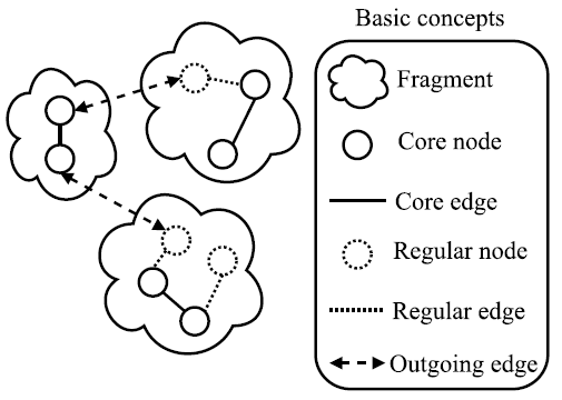
Next, we describe the basic concepts of GHS (See Figure 1]. A fragment is a connected subgraph that belongs to the minimum spanning tree. Fragments can only join via a particular kind of edge, known as the outgoing edge. As a general rule, an outgoing edge has a node that belongs to the fragment and another node that does not. Since a fragment could have more than one outgoing edge, the lowest-weight outgoing edge of a fragment is an outgoing edge whose weight is the lowest. [²] proves that the lowest-weight outgoing edge of a fragment always belongs to the minimum spanning tree. Additionally, the core nodes are the central computing units of the fragment. They find the lowest-weight outgoing edge of a fragment by collecting information about all the outgoing edges. Besides, they initiate the union of two fragments. Finally, the core edge is the one that connects two core nodes.

4. Dynamic Gallager - Humblet - Spira algorithm (DGHS)

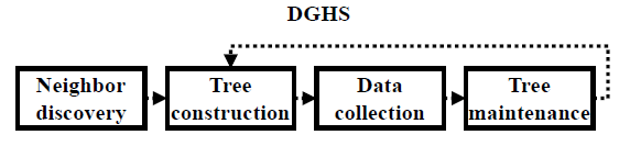
The Dynamic Gallager-Humblet-Spira (DGHS) algorithm builds and maintains a minimum spanning tree. To do so, DGHS is divided into four phases, namely neighbor discovery, tree construction, data collection, and tree maintenance (See Figure 2]. In the neighbor discovery phase, the nodes collect information about their neighbors and the link quality. DGHS defines the link quality as the average number of lost discovery packets. In the tree construction, DGHS finds the minimum spanning tree by executing GHS. In GHS, each node is a different fragment. Subsequently, pairs of fragments merge into a new one. The fragments continue to join until only one remains: the final fragment is the minimum spanning tree. However, this minimum spanning tree is not rooted at the sink. Hence, in the data collection phase, the sink roots the minimum spanning tree at itself by sending a single control message via the branches of the tree. Then, each node starts sending data packets. In the tree maintenance phase, the nodes repair the tree when communication failures occur by merging disconnected fragments. The repair mechanism is initiated by the sink and partially reruns GHS to join disconnected fragments.

Figure 2 Four phases of the Dynamic Gallager-Humblet-Spira algorithm (DGHS) 

4.1 Neighbor discovery

Initially, the nodes do not have any previous knowledge about their neighborhood because they are scattered randomly in the area of interest. So, they collect information about their neighbors and the link quality using a procedure called neighbor discovery. During the neighbor discovery, the nodes periodically broadcast discovery packets with a sequence number. Upon reception of a discovery packet, the nodes compute the link weight which is defined as the average number of discovery packets that have been lost. This computation is done by computing the moving average of sequence number gaps. By exchanging discovery packets, each node maintains a table that includes the link weight for each neighbor.

Specifically, DGHS computes the Exponential Weighted Moving Average (EWMA) of the sequence number gaps. We use EWMA to determine the quality of the links because it applies weights to the samples according to their age. In other words, recent samples strongly influence the resulting average whereas old samples influence the resulting average in a smaller proportion. This property of EWMA is useful in WSNs because it is beneficial to keep an updated neighborhood state which gives more weight to recent samples. We show the definition of EWMA in Equation (1).

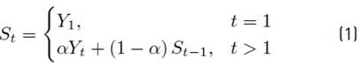
where, Y _t is the input variable (i.e., in this case the sequence number gaps) and α is a constant between [0; 1] that determines the influence of recent and old samples. If α is close to 1 then the resulting average is almost determined exclusively by recent samples; and, if α is close to 0 then the old samples are given more weight. Once the nodes know their neighborhood, the tree construction phase begins.

4.2 Tree construction

DGHS finds the minimum spanning tree by executing GHS. We select GHS because it is a distributed algorithm, it does not require synchronized nodes, it guarantees an execution without deadlocks, it tolerates an unpredictable delay of messages, and it is message-optimal [³]. Hence, GHS is suitable for WSNs. More importantly, GHS is considered the cornerstone algorithm for finding the minimum spanning tree in a distributed manner. So, several algorithms are based on GHS [¹⁹-²¹]. Note that DGHS inherits the advantages of GHS.

Initially, each node belongs to a different fragment. Subsequently, pairs of fragments merge into a new one. To that end, a fragment identifies its lowest-weight outgoing edge and requests the adjacent fragment to join. After accepting the request, the two fragments join into a new one via the lowest-weight outgoing edge. Pairs of fragments continue to join until only one fragment remains: this final fragment is the minimum spanning tree of the graph. Each fragment has a unique name and a level to guide the joining process. The name guarantees that different fragments merge, and the level determines how and when the joining occurs.

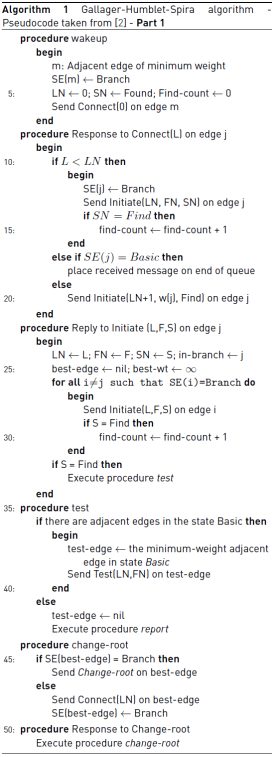
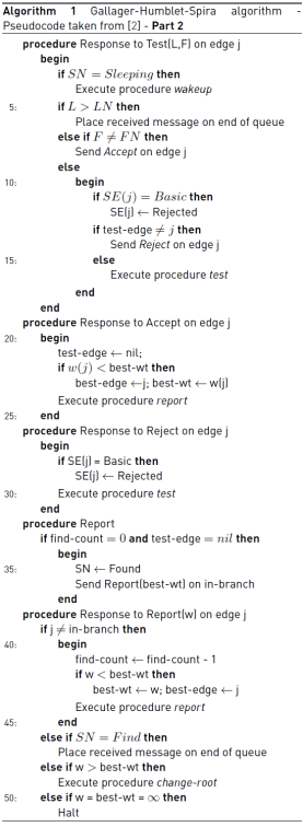
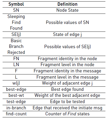
In the remaining of this Subsection, we present in detail the construction of the minimum spanning tree. To that end, we describe the situation where two fragments exchange control messages to join. In other words, we explain a complete round of the tree construction. Note that we included the pseudocode of the minimum spanning tree construction in Algorithm 1 and the nomenclature in Table 2.

Table 2 Nomenclature of GHS 

Before explaining the details of the GHS algorithm, it is necessary to define the states of the nodes and the edges. A node has two states: find or found. In the find-state, the node is examining its edges to find the one which is outgoing and has the lowest weight. Besides, the node is waiting that its children report their lowest-weight outgoing edge. In the found-state, the node has sent to its parent the information about its lowest-weight outgoing edge. Additionally, the node waits for a request to join its fragment with the adjacent one via its lowest-weight outgoing edge; or, it waits for a message informing that the union was completed by another node within its fragment. An edge has three states: basic, branch, and rejected. A basic edge does not specify whether it belongs to the minimum spanning tree or not; a branch edge belongs to the minimum spanning tree; and, a rejected edge does not belong.

Next, we present the details of the GHS algorithm.

In GHS, the nodes send messages, wait for a reply, and process the information. In this way, we describe GHS by introducing its control messages, namely, connect, initiate, test, accept, reject, report, and change root. In the rest of this Section, we employ two fragments to show the message exchange. Suppose a fragment named fn with a node p and level l; and, another fragment named fn′ with a node q and level l′.

At the very beginning of the algorithm, each node is a fragment with name and level equal to zero. Then, the fragments actively seek to join among them. To that end, each fragment finds its lowest-weight outgoing edge and requests the adjacent fragment (i.e., the fragment on the other side of the lowest-weight outgoing edge) to join. At this moment, finding the lowest-weight outgoing edge of the fragment is trivial because it corresponds to the lowest-weight edge of the single node. This is because fragments are composed of a single node, so, all the edges are outgoing, and there are no other nodes which may have a lower-weight outgoing edge. Moreover, a fragment requests another to join by sending a connect message. Suppose fragment fn requests fragment fn′ to join. To that end, node p belonging to the fragment fn sends over the lowest-weight outgoing edge the connect message ⟨connect, l⟩. Upon reception of a connect message, node q belonging to the fragment fn′ responds depending on the level l′ and the status of the edge pq through which the message was received:

• If both fragments have the same level and pq is not a branch edge, then fragment fn′ pospones processing the connect message. This connect message is analyzed again when the level l′ becomes greater than l, or pq becomes a branch edge.

• If both fragments have the same level and pq is a branch edge, then q sends an initiate message to p. Since both fragments are about to join at an equal level, the new fragment gets a new name and level. The name is equal to the weight of the edge pq, and the level is increased by one. Besides, pq becomes the core edge of the new fragment; p and q become core nodes. Moreover, all the nodes in the new fragment go to the find-state. So, the initiate message is ⟨initiate, weight of pq, l + 1, find⟩.

• If the level l′ is greater than l, then q sets the state of the edge qp to branch, and sends an initiate message. Since both fragments are about to join at a different level, the higher-level fragment imposes its name and level over the lower-level fragment. In other words, the lower-level fragment copies the name and level of the higher-level fragment. Thus, the new fragment is called fn′ and has level l′. So, the initiate message is 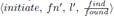. The last parameter is the state of the node q, which can be either find or found, and is represented as . This state is assumed by the nodes in the lower-level fragment.

So, if a fragment requests another to join by sending a connect message, it gets an initiate message in response. This initiate message determines the name, level and state of the nodes in the new fragment. Upon reception of the initiate message , a node updates the name and level of its fragment using fn and l, respectively. Besides, the node assumes the state indicated by the last parameter of the message, and selects the sender of the message as parent. Moreover, the node retransmits the initiate message via its branch edges. By retransmitting this message, all the nodes update the name and level of the fragment; and, they also update the route toward the core nodes.

When a node receives an initiate message and the last parameter is find-state, it changes its state to find. Immediately after the state change, the node starts searching for its lowest-weight outgoing edge. To do that, the node arranges the edges in a weight-ascending list. Then, it sends a test message to the lowest weight edge. In response, the node could receive an accept message, which means that the edge is ougoing. So, the node has found its lowest-weight outgoing edge, and the search is over. On the other hand, the node could receive a reject message, which means that the edge is not outgoing. In this case, the node marks its lowest-weight edge as rejected, and sends a test message to the next edge in the list. If there are no more edges in the list, the node assigns a weight of ∞ to its lowest-weight outgoing edge. For example, suppose that node p is trying to determine whether node q is outgoing or not. To that end, p sends the test message ⟨test, fn, l⟩ to q. Upon reception of the test message, q reacts as follows:

• If the level l is greater than l′, then node q pospones processing the test message. This test message is analyzed again when the level l′ has reached or surpassed l.

• If the level l is lower or equal than l′, then q determines whether it belongs to the same fragment than p. To do that, q compares both fragment names. If fn and fn′ are equal, then q and p belong to the same fragment. Thus, they cannot join. So, q sends a reject message to p, and marks the edge qp as rejected. On the other hand, if fn and fn′ are different, then q and p belong to different fragments. Thus, they can join. So, q sends an accept message to p, and marks the edge qp as lowest-weight outgoing basic edge. In this moment, q has found its lowest-weight outgoing edge: qp.

Once the node has found its lowest-weight outgoing basic edge, it waits for a report message from each child. The report message ⟨report, lwoe⟩ contains the lowest-weight outgoing edge (lwoe) that each child knows. By collecting report messages, the node obtains information about outgoing edges in the fragment and their weights. The node arranges these outgoing edges in a weight-ascending list including its own lowest-weight outgoing basic edge. Subsequently, the node determines that the first element of the list is the lowest-weight outgoing edge. Thus, the node selects the lowest-weight outgoing edge by considering the outgoing edges reported by its children and its own lowest-weight outgoing basic edge. Subsequently, the node informs its parent about its lowest-weight outgoing edge by sending a report message. Once the report message is sent, the node changes its state to found.

The report messages propagate in the fragment from the leaf nodes to the core nodes. When a core node has received a report message from each child and has found its lowest-weight outgoing basic edge, it follows the procedure described above to determine its lowest-weight outgoing edge. However, this lowest-weight outgoing edge is fundamental because it corresponds to the lowest-weight outgoing edge of the whole fragment. If the weight of this outgoing edge is ∞, it means that GHS has found the minimum spanning tree. If the weight is lower than ∞, the core node sends a changeroot message to node p, which originally reported the outgoing edge pq. The core node knows the route towards p because each node remembers the child that reported the best outgoing edge. Upon reception of a changeroot message, node p changes the state of its lowest-weight outgoing edge to branch, and sends a connect message ⟨connect, l⟩ to q.

We are back at the situation where two fragments exchange a connect message to join. Thus, we explained a complete round of the GHS. The tree construction proceeds by joining pairs of fragments until only one remain. It is important to mention that the minimum spanning tree generated by GHS is not necessarily rooted at the sink. Hence, in the next phase, DGHS roots the tree at the sink.

5. Performance evaluation setting

We implement DGHS on Contiki which is a widely used open-source operating system for WSNs. Subsequently, we evaluate the performance of DGHS on Cooja which is the Contiki network emulator. We compare DGHS with a state-of-the-art tree construction mechanism known as LIBP (See Section 2). We use LIBP as a point of reference for the comparison because it outperforms well-known tree construction mechanisms, such as RPL [¹¹] and CTP [²²], regarding power consumption, scalability, throughput, and recovery from failure [⁴].

Table 3 Configuration parameters for the emulations 

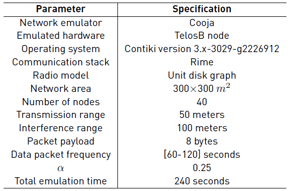
We emulate 40 TelosB nodes in a 300 X 300 m ² area. The nodes are randomly scattered. Regarding the wireless channel, we use the unit disk graph model which assumes that the nodes communicate and interfere in fixed-radius circles. Besides, the transmission range is 50 meters, and the interference range is 100 meters. During the data collection, each node sends a data packet every X seconds, where X is a random number between [60,120] seconds; the packet payload is 8 bytes. We run 20 emulations with different seeds and average the results. Table 3 shows the configuration parameters for the emulations.

We analyze four metrics to evaluate the performance of DGHS:

6. Performance evaluation results

We analyze the number of control packets, energy consumption, convergence time, and memory consumption for DGHS and LIBP.

Figure 3a shows the total number of control packets needed to build a tree using DGHS and LIBP. We see that LIBP uses 25.6% more control packets to construct the tree: LIBP employs 334 control packets, and DGHS uses 266. We expected that DGHS uses a lower number of control packets because it is based on GHS which is message-optimal. On the other hand, LIBP constructs the tree by sending periodic beacons and ACKs. This periodic approach does not limit the number of control packets resulting in unnecessary transmissions. Other tree construction mechanisms, such as RPL [¹¹] and CTP [²²], implement an adaptive beaconing called the Trickle algorithm [²³]. The Trickle algorithm determines the sending rates of beacons in such a way that it sends control packets more often when there are network changes, and it reduces the control traffic rates when the network stabilizes. To do that, the Trickle algorithm uses timers that control the sending rates of beacons. The Trickle algorithm determines the value of the timer by choosing a random value between [I/2,I] where I is initially defined as I _min . When the timer expires, RPL sends a beacon and duplicates the value of I up to I _max . Additionally, the timer is reset to I _min when RPL detects an inconsistency in the network. By setting I _min to a few miliseconds and I _max to 1 hour, the Trickle algorithm can reduce the control traffic up to 75% compared to sending a beacon every 30 seconds [²⁴].

Figure 3 Performance evaluation results 

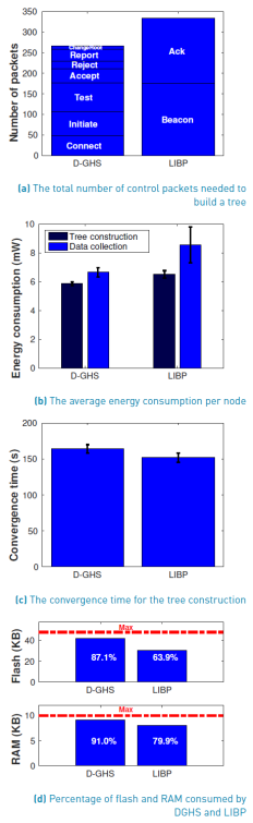
Figure 3b shows the average energy consumption per node during the tree construction and the data collection. During the tree construction, DGHS consumes 9.2% less energy than LIBP: each node running DGHS consumes 5.9mW on average, and each node running LIBP consumes 6.5mW on average. DGHS consumes less energy than LIBP during the tree construction because it uses fewer control packets. So, the fact that DGHS is based-on a message-optimal algorithm leads to energy savings. During the data collection, DGHS consumes 22.1% less energy than LIBP: each node running DGHS consumes 6.7mW on average, and each node running LIBP consumes 8.6mW on average. DGHS consumes less energy than LIBP because the nodes send the data packets via optimal paths. Remember that DGHS routes the packets via the minimum spanning tree which includes the optimal paths. On the other hand, LIBP routes the data packets via sub-optimal paths causing higher energy consumption. Hence, DGHS is more energy-efficient than LIBP during the tree construction and the data collection. Note that the major energy savings occur in the data collection where the network spends most of the time. So, the long-term energy saving is significant since DGHS could increase the network lifetime by around 22.1%.

Figure 3c shows the convergence time for the tree construction in DGHS and LIBP. We see that DGHS converges 8.1% slower than LIBP: it converges after 164.1 seconds, and LIBP does after 151.8 seconds. The higher convergence time of DGHS is due to the delay of sending information from the outgoing edges to the core nodes using a multi-hop approach. Remember that the core nodes collect information from the whole fragment and determine which is the lowest-weight outgoing edge. So, the higher convergence time of DGHS is because sending information to the core nodes via multiple hops is time-consuming. On the contrary, in LIBP, the nodes rely exclusively on information from their one-hop neighbors. Hence, they avoid sending information over multiple hops resulting in lower convergence time. In this way, DGHS relies on information provided by neighbors that are N-hops away (note that the value of N is determined by the size of the fragment). On the contrary, LIBP relies on information provided by 1-hop neighbors. So, the delay of packets traversing N-hops increases the convergence time of DGHS. Note that this convergence time is typical of mechanism that gather complete information about the neighborhood by sending packets through N-hops. So, increasing the convergence time is the price paid for having complete information of the neighborhood that results in the optimal paths found by DGHS.

Figure 3d shows the percentage of flash and RAM consumed by DGHS and LIBP on the TelosB nodes. We see that DGHS slightly consumes more memory than LIBP: it consumes 23.2% more flash and 11.1% more RAM. The higher memory consumption of DGHS is because it requires seven types of control messages and LIBP only requires two. The additional control messages of DGHS employ additional structures, lists, and validations causing a higher memory consumption. This result was expected since DGHS can find the minimum spanning tree, so, it is more complex than a protocol that finds a sub-optimal tree such as LIBP. It is important to mention that the flash and RAM usage of DGHS is near to the maximum. DGHS consumes 41.8KB out of 48KB of flash (i.e., 87.1%), and 9.1KB out of 10KB of RAM (i.e., 91.0%). So, DGHS implementation has little space to add new functionalities. A straightforward solution to this problem is to use a node with more memory resources. For example, the RE-Mote (manufacturer Zolertia) has 512KB of flash and 32KB of RAM; the wismote (manufacturer arago-systems) has 256KB of flash and 16KB of RAM. In this way, implementing DGHS in those nodes would leave room for plenty of new functionalities such as adding IPv6.

7. Conclusions and future work

We propose the DGHS algorithm which builds and maintains a minimum spanning tree. To do so, DGHS is divided into four phases, namely neighbor discovery, tree construction, data collection, and tree maintenance. We evaluate the performance of DGHS on Cooja, which is the Contiki network emulator. The results show that DGHS uses 25.6% fewer control packets than LIBP during the tree construction. Besides, DGHS consumes on average less energy that LIBP: it consumes on average 0.6mW less during the tree construction, and 1.9mW less during the data collection. However, DGHS slightly increases the memory size and convergence time because of its higher complexity. In conclusion, DGHS reduces the number of control messages and the energy consumption, at the cost of a slight increase in memory size and convergence time. In future work, we plan to design a fault detection mechanism that triggers the tree maintenance phase, instead of searching for disconnected sub-fragments periodically. We also plan to evaluate DGHS on a testbed to consider the challenges of a real communication channel.