


 Inglês (pdf)
 Artigo em XML
 Referências do artigo
 Enviar este artigo por email
 Citado por SciELO
  Citado por Google
  Similares em
SciELO
Similares em
SciELO  Similares em Google
 Permalink
I. INTRODUCTION
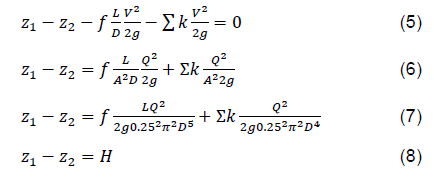
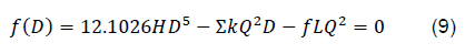
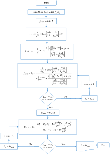
In the design of hydraulic systems, the calculation of the diameter is fundamental. This parameter determines the behavior of the pressure along the pipe. Likewise, the average flow velocity will remain constant because there is no variation in the pipe cross-section. This effect causes the system to have a single value for the friction coefficient and Reynolds number. The design equation for single pipe diameters (9) is obtained by accepting the governing equation for pressure-flow (2) and setting the flow velocity in terms of the flow rate. This fifth-degree equation presents two unknowns, the diameter and the friction coefficient. Therefore, a nested loop must be established to solve both variables simultaneously. For the diameter, it is suggested starting from a seed value equal to 0.254 m, and for the friction coefficient, the recommended seed value is 0.015. These values accelerate the convergence processes of the numerical method used. Once the corresponding diameter is found, it should be approximated to the upper commercial diameter. Consequently, if a single pipe is considered, which connects two reservoirs (Figure 1) and applies the Energy Equation (1) on the surface of the reservoirs, it is obtained.
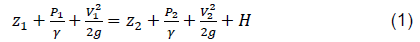
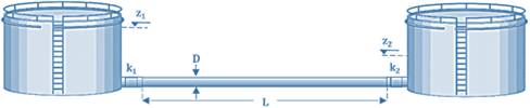
For a constant incompressible one-dimensional flow, the energy per unit weight (Nm/N) generated by the hydraulic system (Figure 1) is defined by the Energy Equation (1); where tank 1 has: z1position head (m),
 : pressure head (m),
 : velocity head (m), H: head loss (m). The head loss H is determined by the losses caused by the friction between the pipe and the fluid; the losses generated by the fittings. The Darcy-Weisbach equation (2) rules the head loss.
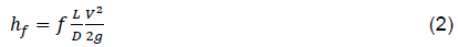
Where, h f : head loss (m); f: friction coefficient; L: piping length (m); D: diameter (m); V: average flow velocity (m/s); g: gravity (m/s2). For local or minor losses, we have,
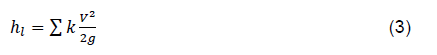
Where, h l : minor losses (m); k: minor loss coefficient (dimensionless); V: average flow velocity (m/s); g: gravity (m/s2). The principle of conservation of mass for a given control volume, where the flow has an incompressible performance and there is no variation of the discharge as a function of time and space (steady-state), is determined by the principle of continuity from the following expression:

Where, Q: Discharge (m3/s); V: Average flow velocity (m/s); A: Cross-sectional area of the pipe (m2).
Thus, from the energy equation (1) and establishing the velocity in terms of the streamflow, we have:
Design equation:
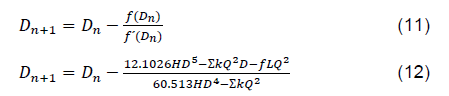
First derivative:

Newton-Raphson method:
The nested loop development (Figure 2) determines the solution of the equation (9). For the single pipes diameter calculation, 75% of the total head loss of the system is proposed as a seed value for the friction losses [1]. For this study, the input signals correspond to Q: discharge (m3/s), H: head loss (m), L: pipe length (m), ε: pipe roughness (m), 𝜗: kinematic viscosity (m2/s), and Ʃk: summation of minor loss coefficients (dimensionless). The output signal is determined by the diameter (m). The equation proposed by Colebrook-White (13) was implemented to calculate the friction coefficient (f).
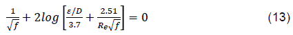
Where f: coefficient of friction (dimensionless factor), ε: absolute roughness (m), D: diameter (m), Re: Reynolds number (dimensionless factor). Similarly, the Newton-Raphson method for the calculation of the friction coefficient is given by:
If two tanks connected by a pipe section are considered (Figure 1), and the total head loss and the discharge conveyed by the pipe are known, it is possible to determine the value of the internal diameter from equation (9). Likewise, [2] used the Fixed-Point iteration method to calculate the diameter in pressurized piping systems. Figure 2 presents the flowchart for the nested loop with two unknowns and six input signals; the process achieves convergence with an approximation equal to 1E-12.
II. Neuronal Structure
A. Data Processing
Using Visual Basic (®Excel), a routine is structured to calculate the diameter (D) from the input signals (Q, H, L, ε, 𝜗, Ʃk). The code is created from equations (12) and (14). The iteration shown in Table 2 was repeated 5,000 times from random data fitting a normal distribution, establishing the input-output matrix for this study. These data are available at the following link (download data). The Domain of the input variables varies from minimum to maximum values; Table 1 shows the ranges established.
Table 1 Input variable ranges (inputs).
| Discharge | Head Loss | Length | Roughness | Kinematic viscosity | Coef. accessory | |
|---|---|---|---|---|---|---|
| Q (m3/s) | H (m) | L (m) | ε (m) | Vis (m2/s) | Ʃk | |
| Minimum | 0.000096 | 10 | 100 | 0.0000015 | 0.000000661 | 0 |
| Maximum | 0.475 | 50 | 500 | 0.00045 | 0.000001519 | 10 |
The following code made in Visual Basic (®Excel) generates an iterative loop for the diameter and the friction coefficient. The seed values directly affect the convergence process. In this sense, 0.015 is the seed value for the friction coefficient and 0.254 m for the diameter. If the seed values are far from the solution value, there is a probability that the algorithm will diverge. Consequently, the proposed seed values guarantee the convergence of the iterative method. The code outputs 200 iterations for each diameter value and friction coefficient with an approximation of 1E-12 for the objective function. The loop stops when it does not detect a numerical value in the following grid cell to be iterated.
Dim i As Integer
Sub MacroD_f()
For i = 1 To 10
Range("h11").Select
Do Until ActiveCell = ""
ActiveCell.Offset(0, 1).GoalSeek Goal:=0, ChangingCell:=ActiveCell
ActiveCell.Offset(1, 0).Range("A1").Select
Loop
Range("o11").Select
Do Until ActiveCell = ""
ActiveCell.Offset(0, 1).GoalSeek Goal:=0, ChangingCell:=ActiveCell
ActiveCell.Offset(1, 0).Range("A1").Select
Loop Next i
End Sub
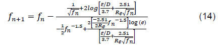
Table 2 shows the results generated for the diameter calculation from the nested loop. In order to explain the velocity as a discharge function and consider the input data for head loss, pipe length, discharge, and the seed friction coefficient, a fifth-degree equation is established. The initial equation solution determines the value of the cross-sectional pipe area. Consequently, it is possible to calculate the flow velocity. Once the speed is calculated, the Reynolds number and the estimated friction coefficient are obtained. Then, the loop is generated until convergence of the objective function is reached, both for the diameter and the friction coefficient simultaneously. Usually, this convergence is reached in the fourth iteration with an approximation equal to 1E-12. The method used to obtain the training signals for this study corresponds to the numerical approach proposed by Newton-Raphson (12), (14).
Table 2 Initial iteration of input signals.
| f | Q (m3/s) | H (m) | L (m) | Ʃk | D (m) | V (m/s) | υ (m2/s) | Re | ε (m) | f´ |
| 1.500E-02 | 3.190E-01 | 5.0008E+01 | 1.887E+02 | 8E+00 | 2.40E-01 | 7.04E+00 | 1.416E-06 | 1.194E+06 | 3.24E-04 | 2.135E-02 |
| 2.135E-02 | 3.190E-01 | 5.0008E+01 | 1.887E+02 | 8E+00 | 2.52E-01 | 6.39E+00 | 1.416E-06 | 1.138E+06 | 3.24E-04 | 2.111E-02 |
| 2.111E-02 | 3.190E-01 | 5.0008E+01 | 1.887E+02 | 8E+00 | 2.51E-01 | 6.41E+00 | 1.416E-06 | 1.140E+06 | 3.24E-04 | 2.112E-02 |
| 2.112E-02 | 3.190E-01 | 5.0008E+01 | 1.887E+02 | 8E+00 | 2.51E-01 | 6.41E+00 | 1.416E-06 | 1.140E+06 | 3.24E-04 | 2.112E-02 |
B. Data Scale
We, as authors, chose to perform the neural model with the actual data without scaling. Table 3 establishes that the statistical criteria are more favorable for the unscaled data than the scaled data from the logarithm in base 10.
C. Artificial Neural Network (ANN) Architecture
Due to the nonlinearity of the functions that estimate the diameter (12) and the friction coefficient (14), it is feasible to estimate the output parameter through optimization algorithms. Artificial neural networks can approximate any continuous nonlinear function independent of the function degree [4]. The implementation of artificial intelligence techniques contributes to finding the minimum error surface generated by the cost function. A neural structure created in Matlab (2021a) is proposed (Figure 3) corresponding to 6 input signals (Q, H, L, ε, 𝜗, Ʃk), a hidden layer with 25 neurons, and an output signal for diameter estimation. The logsig transfer function showed optimal results in terms of MSE and computational time required to reach convergence. The Levenberg-Marquardt (trainlm) method is suited to both the training data and the test data sets. The network weights are iteratively adjusted from the error estimate [5] [6] describes the application of the Levenberg-Marquardt in neural network systems for training. This algorithm has demonstrated a higher training speed for the neural network [7]. Similarly, [8] proposes a neural architecture of 5 input variables, a hidden layer with 36 neurons, and 10 output parameters to classify the optimal commercial diameter for the hydraulic system.
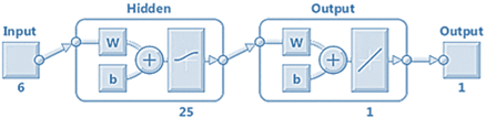
Table 4 indicates different neural structures tested for this study to obtain the lowest value for the MSE; this value was achieved for the architecture (6-25-1) with an MSE equal to 5.41E-6. It was found that increasing the number of hidden layers does not guarantee a decrease in the MSE, and as a consequence, it does increase the computational cost of the iterative process. The computational time for the (6-25-25-25-1) scheme was 3 hours and 25 minutes. In contrast, the time required for the (6-25-25-1) scheme was 15 minutes. Thus, neural models with several hidden layers tend to overfit so that the model can predict the training data. However, for the prediction of independent data, the overfitted neural model has shortcomings. The most important property of a neural network is its ability to generalize and model new input data [9].
Table 4 Network topology for diameter calculation [logsig, trainlm].
| No. of hidden layers | No. of neurons per layer | Architecture | R2 | MAE | MSE | SSE | SAE | BCE |
| 1 | 2 | 6-2-1 | 9.84E+0 | 6.16E-03 | 7.64E-5 | 3.82E-1 | 30.3E+00 | 15 E+00 |
| 1 | 10 | 6-10-1 | 9.99E+0 | 1.67E-03 | 9.74E-6 | 4.87E-2 | 4.95E-02 | 4.63E-01 |
| 1 | 20 | 6-20-1 | 9.99E+0 | 1.28E-03 | 7.68E-6 | 3.84E-2 | 6.41E+00 | 4.47E-01 |
| 1 | 25 | 6-25-1 | 9.99E+0 | 9.71E-04 | 5.41E-6 | 2.71E-2 | 4.84E+00 | 1.25E+00 |
| 1 | 30 | 6-30-1 | 9.99E+0 | 9.96E-04 | 5.65E-6 | 2.82E-2 | 4.97E+00 | 8.54E-01 |
| 2 | 10 | 6-10-10-1 | 9.99E+0 | 9.11E-04 | 5.85E-6 | 2.93E-2 | 4.55E+00 | 1.48E-01 |
| 2 | 30 | 6-30-30-1 | 9.99E+0 | 1.08E-04 | 6.39E-6 | 3.19E-2 | 5.39E+00 | 2.25E-01 |
| 3 | 25 | 6-25-25-25-1 | 9.99E+0 | 1.09E-03 | 6.63E-6 | 3.31E-2 | 5.46E+00 | 2.17E-01 |
D. Neural Network Training
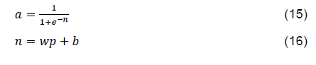
The Levenberg-Marquardt training function (trainlm) uses the second derivatives of the cost function upgrading the convergence times [10]. The implementation of this algorithm is feasible as long as the second derivative of the neural network weights exists. Thus, the input signals are affected by the random weights and biases values (16). Once this value is obtained, the log-sigmoid activation function (logsig) (15) is implemented. This function implements the Jacobian matrix for the calculations. This matrix is formed by the first-order partial derivatives of the function. The performance for this function is measured through the MSE. The algorithm presents good performance for escaping moderate local minima and oscillation problems. The interval [0,1] determines the range of the corresponding function.
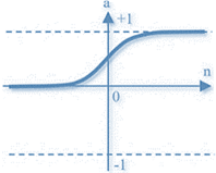
The following expression defines the log-sigmoid activation function (logsig):
Six neural architectures are proposed for the diameter in pressure piping systems calculation. The lowest Pearson Correlation Coefficient was obtained for the scheme (6-2-1) with an R equal to 0.99282; the computational time required for this scheme was 4 minutes. Figure 5a presents the dispersion of the outputs for ANN (6-2-1). However, for the arrangement (6-25-1), represented in Figure 5d, an R equal to 0.99939 indicates the best training and output signals fit; the computational time required was approximately 10 minutes. The scheme (6-30-30-1) presented a similar performance to the system (6-25-1). Nevertheless, this scheme composed of two hidden layers considerably increased the computational time required to reach convergence, approximately 3 hours and 25 minutes.
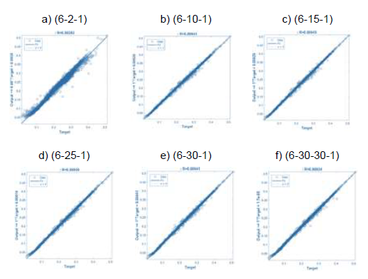
Figure 6 shows the 3D irregular surface structured from the weights, the bias parameter, and the sum of squared errors. The objective of the cost function is to establish the minimum for this surface.
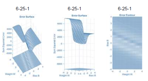
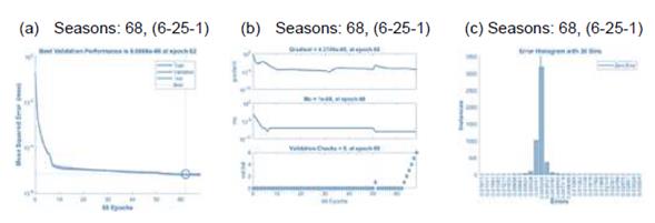
Figure 7a indicates the performance of the validation and training curve; the error decreases as the number of epochs of the iterative process increases. If the MSE of the validation curve starts to increase and distance itself from the training curve, the model will overfit, which directly affects the generalization capability of the network. Figure 7b presents the adaptation parameter mu used in the Levenberg-Marquardt optimization process. For this study, the mu parameter corresponds to 1E-08 for season 68.
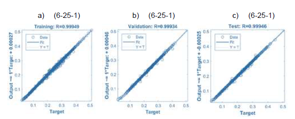
The data were divided into three sets using random indexes, training, validation, and test, as represented in Figure 8. The straight line at 45° represents a perfect fit, i.e., the values of the estimated outputs are equal to the target values. Figure 8c indicates the relationship between outcomes and targets for the test set. This study found a linear relationship between the output signals and the objectives with a Pearson Correlation Coefficient equal to 0.99946 for a neural scheme (6-25-1).
E. Validation
For the analysis of the network output signal and to validate the independent data set, six statistics were considered: R (Pearson correlation coefficient), MAE (Mean Absolute Error), MSE (Mean Squared Errors), SSE (Sum of Squared Errors), SAE (Sum of Absolute Errors), BCE (Binary Cross Entropy). In order to establish a representative spectrum associated with the independent data set, a set of 1,000 random data was structured for the test signals. Cross-validation allows comparing the estimated signals with the target values from the independent data of the training set. The error histogram presented in Figure 7c indicates a minimum standard deviation with a mean tending to zero for the individual data; the histogram tends to be symmetric around the average. The percentage difference of the MSE between the training data and the independent data corresponds to 0.00015%, indicating the generalization capability of the neural model.
Table 5 Cross-validation
| Data | No. of data | Architecture | R2 | MAE | MSE | SSE | SAE | BCE |
| Training | 5,000 | 6-25-1 | 9.99E+00 | 9.71E-04 | 5.41E-6 | 2.71E-2 | 4.84E+00 | 1.25E+00 |
| Independent | 1,000 | 6-25-1 | 9.98E+00 | 1.27E-03 | 6.91E-06 | 6.91E-03 | 1.27E+00 | 0.52E-01 |
The U.S. Environmental Protection Agency developed ®Epanet for the calculation of pressurized piping systems. This system works with hydraulic simulation periods from the drinking water distribution systems. It also models water quality within a pressurized network and can be used for any non-compressible fluid flowing under pressure analysis. ®Epanet determines the flow rates through the pipes and the values of the pressures at the nodes based on the principle of conservation of mass and energy by implementing the gradient method proposed by Todini and Pilati (1987). For the calculation of friction losses, three models are presented: Darcy-Weisbach (D-W), Hazen-Williams (H-W), Chézy-Manning (C-M).
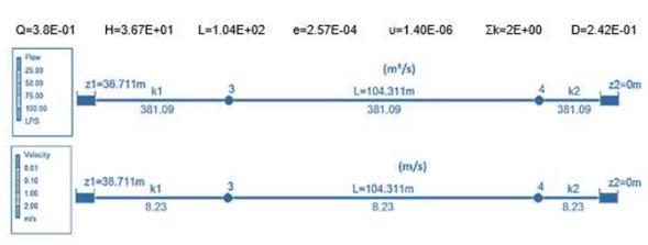
Similarly, the neural network was evaluated from the data shown in Table 6. The results obtained were compared with the values calculated in ®Epanet, ®Excel, and the application for the calculation of pressure pipes of the hydraulics online website, accepting the Darcy Weisbach equation (2). For the first data in Table 6, the modeling was performed in ®MatLab software. Two tanks were established (Figure 1), the first tank with a height above the water surface equal to 36.712 m, a fitting at the inlet with a coefficient of 1, the main pipe with a diameter of 0.2428 m, a length equal to 104.31 m, a loss coefficient per fitting equal to 1 at the outlet, a tank at the end with zero height, the kinematic viscosity corresponds to 0.000001404 m2/s, and the roughness of the pipe equals to 0.0002574 m. The model in ®Epanet obtained a flow rate equal to 0.38109 m3/s, with a velocity of 8.23 m/s. The results obtained in ®Epanet, ®Excel, and the website validate the values calculated by ANN (6-25-1). According to the hydraulic calculation performed in ®Epanet, the velocity remains constant because the system does not present a variation of the pipe cross-section. This performance causes the Reynolds number and the friction coefficient to remain constant along the length of the pipe.
Table 6 ANN validation, Epanet, Excel, and web page.
| Input | Output | |||||||||
| # | Q (m3/s) | H (m) | L (m) | e (m) | υ (m2/s) | Ʃk | Diameter (m) | |||
| RNA (6-25-2) | ®Epanet | ®Excel | Página Web (www.edgarladino.com) | |||||||
| 1 | 3.81E-01 | 3.67E+01 | 1.04E+02 | 2.57E-04 | 1.40E-06 | 2E+00 | 2.42E-01 | 2.42E-01 | 2.42E-01 | 2.42E-01 |
| 2 | 4.6588E-01 | 3.19E+01 | 1.05E+02 | 1.46E-04 | 1.39E-06 | 3E+00 | 2.72E-01 | 2.71E-01 | 2.71E-01 | 2.71E-01 |
| 3 | 1.618E-01 | 1.31E+01 | 1.33E+02 | 4.74E-05 | 1.24E-06 | 4E+00 | 2.17E-01 | 2.16E-01 | 2.16E-01 | 2.16E-01 |
| 4 | 2.392E-01 | 1.10E+01 | 1.01E+02 | 1.83E-04 | 1.13E-06 | 2E+00 | 2.52E-01 | 2.52E-01 | 2.52E-01 | 2.52E-01 |
| 5 | 3.535E-01 | 3.03E+01 | 1.55E+02 | 2.35E-04 | 7.76E-07 | 9E+00 | 2.85E-01 | 2.84E-01 | 2.84E-01 | 2.84E-01 |
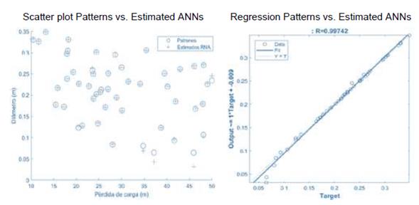
In addition, the generalization capability of the neural model is evidenced by the estimation of 50 independent data. These data show no dependence on the training, test, and validation data set. Figure 10 shows the actual data (circles) obtained from equations (12), (14), and the ANN estimated data (crosses). The Pearson Correlation Coefficient obtained was equal to 9.9742E-1 showing a linear relationship between the input signals and the estimated signals. The root average squared error for the 50 data corresponded to 3.65E-05. The cross-entropy obtained was equal to 5.504E-1, which establishes a lower uncertainty for the probability distribution.
Finally, Figure 10 shows the generalization capability of the neural network (6-25-1) to estimate the theoretical diameter in pressurized pipes. This study demonstrated the potential of artificial neural networks to solve nonlinear systems.
III. CONCLUSIONS
The best performing architecture corresponded to a hidden layer with 25 neurons (6-25-1), presenting an MSE equal to 5.41E-6 and 9.98E+00 for the Pearson Correlation Coefficient. The cross-validation of the neural scheme was performed from 1,000 independent input signals of the training set, obtaining an MSE equal to 6.91E-6. This validation demonstrated the generalization capability of the proposed neural arrangement for the theoretical diameter in pressurized piping systems estimation.
It was found that increasing the number of hidden layers does not guarantee a decrease in the MSE and increases the computational cost of the iterative process. Similarly, increasing the number of hidden layers and neurons can generate overfitting of the input signals, limiting the model’s capacity in the generalization process. Finally, this study demonstrated the potential of artificial neural networks to solve nonlinear systems.

