English (pdf)
 Article in xml format
 Article references
 Send this article by e-mail
 Cited by SciELO
  Cited by Google
  Similars in
SciELO
Similars in
SciELO  Similars in Google
 Permalink
INTRODUCTION
A fundamental issue closely related to asset allocation and risk management is the increasing of interdependence in financial markets during crisis episodes. There is a common concern related to the fact that disequilibrium generated in one region is extended to a wide range of markets and countries, and fundamentals are not enough to explain these changes. Dependence phenomenon started to be measured and studied after the crisis in the 1990s by using correlation analysis, often based on ARCH type models (Hamao, Masulis, & Ng, 1990; King & Wadwhani, 1990; Lin, Engle, & Ito, 1994; Malliaris & Urrutia, 1992; Susmel & Engle, 1994).
Exchange rate is a key financial and economic variable. Since 1970 (after the abandonment of the gold standard), relative currency prices have been fluctuating, and countries have experienced periods of instability and constant depreciations (appreciations) associated with crises. In this sense, the exchange rates returns experiences similar behaviour when financial disequilibria occurs. Financial literature has identified this phenomenon as: asymmetric dependence. Asymmetric dependence is displayed when two returns exhibit greater correlation during market downturns than market upturns. A possible explanation could be because investors are more uncertain about state of the economy (Patton, 2006).
Asymmetric dependence between exchange rates could come from portfolio rebalancing or could be explained by Central Banks' differentiated responses to exchange rate movements. For example, to guarantee trade competitiveness, if country A observes that the currency of country B is depreciating, and both countries are commercial rivals; country A's Central Bank will intervene to ensure a matching depreciation between the currency of country A and B. In other words, currencies from country A and B will depreciate in the same magnitude, in relation to the currency of the common business partner. Changes in these variables are translated into higher volatility for both currencies. Thus, dependence level could be higher during high volatility periods than during low ones (Patton, 2001).
Evidence of the non-normality in distributions of many common economic and financial variables has been widely reported. These kinds of variables exhibit stylized facts including: skewness, kurtosis (peaked and heavy-tailed distributions), non-linearity, long run memory (shocks effects remain during long time), leverage effect (good news has lower impact than bad in volatility), and asymmetric dependence. To overcome difficulties in financial variables estimation, this paper proposes using ARCH models as a suitable approach to capture time-varying behaviour of series. In terms of measuring the strength of linkages between financial variables, Copula is a more informative measure of dependence between two (or more) variables than linear correlation.
This paper analyses bivariate asymmetric dependence in the exchange rate volatility of: the British Pound, Japanese Yen, Euro, and Mexican Peso in comparison to the U.S. dollar during four sub-periods: 1994-1999, 2000-2007, 2007-2012, 20132018, which are characterized by the presence of turmoil and then subsequent periods of calm. To achieve this goal, univariate GARCH and TARCH models are employed to estimate conditional volatility of series. Once conditional variance is modelled, a Copula approach is used to measure volatility dependence and tail volatility dependence by currency pairs. Tail dependence results allow us to determine whether there is higher dependence during high volatility episodes.
This article makes two contributions. First, it proposes a relatively innovative methodology to analyse asymmetric dependence in a market to which not much attention has been paid: the exchange rate market. Second, it provides valuable information about the dependence structure of currency prices, which promotes better investment strategies in terms of asset allocation, pricing, and risk management.1 Related to monetary policy, policy-makers could use this information to anticipate Central Bank decisions and have a better market response, avoiding disequilibria in other markets and loss of commercial competitiveness.
The structure of this paper is the following: section 2 presents the literature review, section 3 develops the methodology and data used, section 4 analyses empirical evidence, and section 5 concludes the paper.
LITERATURE REVIEW
Copula is an approach which overcomes the limitations of traditional methodologies, and captures non-linearity, non-normality, skewness, and asymmetry in joint distributions without considering which distributions financial series exhibit.
Due to the advantages of copula, there is a growing body of literature on the approach (Arreola Hernandez, Hammoudeh, Nguyen, Al Janabi, & Reboredo, 2017; Bouri, Gupta, Lau, Roubaud, & Wang, 2018; Liu, Long, Zhang, & Li, 2019 are some examples).
Closely related with this research, recently, academia has focused on research about dependence in heavy tail distributions. Yao and Sun (2018) study tail dependence structure between policy uncertainty and financial markets; their results show changes in tail dependence structure across time and regime switching behaviour. Boako, Tiwari, Ibrahim, and Ji (2018) analyse tail dependence between gold and stock markets. They identify co-jump phenomenon and conclude that there is a positive dependence between the markets.
Asymmetric dependence is an interesting topic, and several studies have been undertaken about this phenomenon on different assets, but especially on stock markets. Longin and Solnik (2001) test the hypothesis of increasing equity market correlation in volatile times. They use Extreme Value Theory to model the Multi-variate Distribution Tails and measure extreme correlation. Empirical results show that correlation increases in bear markets but not in bull markets.
Patton (2004) analyses two types of asymmetries in joint distributions: skewness in individual stock market distribution and asymmetry in dependence between stocks. The study measures the importance of these two asymmetries in terms of asset allocation. Evidence reveals that, for investors with no short-sales constraints, knowledge of higher moments and asymmetric dependence leads to gains that are economically significant and statistically significant in some cases.
Kenourgios, Samita, and Paltalidis (2011) study asymmetric dependence in BRICS and U.S. and U.K. stock markets, employing a multivariate regime-switching Gaussian copula model and the asymmetric generalized dynamic conditional correlation. Findings suggest a contagion effect from the crisis country to all others.
A vast amount of literature about extreme dependence estimated by copulas, between stock markets and oil price, has recently been developed. Among these studies are: Kocaarslan, Sari, Gormus, and Soytas (2017), Mensi, Hammoudeh, Shahzad and Shahbaz (2017), Li and Wei (2018), Ji, Liu, Zhao, and Fan (2018), and Shahzad, Mensi, Hammoudeh, Rehman, and Al-Yahyaee (2018).
In terms of asymmetric dependence on exchange rate estimated by copulas, the literature is scarcer than that on about equity markets. Patton (2001 and 2006) test for asymmetry in a model of dependence between the Japanese Yen and the Deutsche Mark. Both articles find that the mark-dollar and yen-dollar exchange rates are more correlated when they are depreciating against the dollar than when they are appreciating.
Closely following Patton's research, this paper aims to analyse the asymmetry in exchange rate volatility dependence between the British Pound, Japanese Yen, Euro, and Mexican Peso compared to the U.S. dollar. The difference with Patton's studies, in terms of variables, is that, in this article, dependence is modelled on volatility, instead of on returns. Methodologically, there are also numerous differences. In this study, symmetric and asymmetric GARCH models are used to estimate conditional volatility. Then, copulas are used to measured tail dependence on volatility (by pairs). Upper and lower tail dependence parameters confirm whether exchange rate dependence is higher during episodes of turmoil.
DATA AND METHODOLOGY
Data
This paper uses daily exchange rate data (LCU/USD) from four currencies: the British Pound, Japanese Yen, Euro, and Mexican Peso. The series go from 1994 to 2018 and are divided into sub-periods, according to episodes of calm and turmoil: 1994-1999, 2000-2007, 2007-2012, 2013-2018.2 Descriptive statistics are presented in Table 1.
Table 1 Descriptive Statistics Exchange Rate Returns Series
| EURO | POUND | PESO | YEN | |
|---|---|---|---|---|
| Mean | -1.48E-06 | 2.48E-05 | 4.84E-06 | 0.000292 |
| Median | 0.0000 | -0.0001 | 0.0000 | 0.0001 |
| Maximum | 0.0474 | 0.0816 | 0.2016 | 0.0399 |
| Minimum | -0.0439 | -0.0389 | -0.1797 | -0.0724 |
| Std. Dev. | 0.0063 | 0.0057 | 0.0100 | 0.0069 |
| Skewness | -0.1122 | 0.6414 | 2.9340 | -0.5454 |
| Kurtosis | 6.0259 | 13.4805 | 93.2160 | 8.8791 |
| Jarque-Bera | 2416.7 | 29265.0 | 2145505.0 | 9385.2 |
Source: Own elaboration.
The non-normality of the data is apparent from the coefficients of skewness and kurtosis. Also, the Jarque-Bera test (reported in the last line of the table) strongly rejects normality.
Methodology
GARCH Model
ARCH models (Autoregressive Conditional Heteroscedasticity), GARCH, and all the extensions have been identified in the empirical literature as effective as they model the volatility of financial series. This is because GARCH models capture some features of asset returns volatility flows. Among these stylized facts are: thick tails, volatility clustering, leverage effects, accumulative information in non-trading periods, strong inverse relations between volatility, and serial correlation and co-movements in volatilities (Bollerslev, Engle, & Nelson, 1994).
Based on the GARCH approach's effectiveness and good fit on modelling asset prices volatility, this paper uses them to analyse whether dependence increases between exchange rates during high volatility periods.
Daily returns are identified as the difference in the natural logarithm of the exchange rate for the two consecutive trading days;
R t = log (IPC )(t )- log(lPC )(t-1) (1)
Unit root tests are applied to prove the presence stationarity in individual financial series. Therefore, the Augmented Dickey Fuller test is used, where, for a return series Rt, the ADF consists of a regression of the first difference of the series against the series lagged k times as follows:
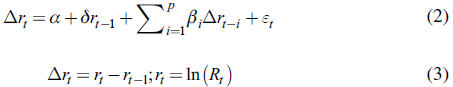
The null hypothesis is H 0 : δ = 0 y H 1 : δ < 1. The null hypothesis acceptance means that the series has a unit root.
GARCH modelling (Bollerslev, 1986; Taylor, 1986) assumes conditional heteroscedasticity with homoscedastic unconditional error variance. The changes in variance are functions of the realizations of preceding errors and of the squared disturbances (Casas & Cepeda, 2008). Thus, the conditional variance of GARCH (p,q) is specified as follows:
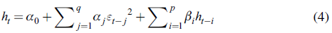
With α 0 > 0, α 1 , α 2> ... α q ≥ 0 y β 1 , β 2 , β 3 ,... β q ≥ 0 to ensure the conditional variance is positive, h t represents the conditional variance estimated with the relevant past information; β i . are the lagged GARCH coefficients, which indicates that changes in the conditional variance disappear slowly. In other words, this shows volatility persistence; α j . is the error coefficient. If it takes high values, it means that there is a high sensibility of the volatility related to market movements. If (α+ β) value is near but lower than the unit, it means that a shock at time t will persist in future periods. Being near to the unit implies that series has long memory (Joshi, 2012). This GARCH model is also known as symmetric because it considers that negative and positive variations have the same impact on volatility. The model is then tested for the ARCH effect using ARCH-LM test. If the coefficient is not statistically significant, the model will be adequate.
TARCH Model
There is a high variety of asymmetric GARCH models: EGARCH de Nelson (1991), GJR-GARCH (Glosten, Jagannathan, & Runkle, 1993), T-GARCH (Zakoian, 1994), APARCH (Ding et al., 1993), PNP- GARCH (Bae & Karolyi, op cit.) or T- GARCH (Hsin, 2004) are just a few.
The TARCH model proposed in this paper has the following generalized specification of the variance equation:

Where d t = 1 if ε t < 0
In this model, if ε t-i > 0, the positive residual values are interpreted by positive shocks. If ε t-i < 0 , the negative residual values are represented as negative shocks. The positive news has an a1 impact and negative news has a α1 + γ j effect. Whether γ 1 > o, negative news increases volatility, this effect is known as asymmetric volatility or leverage effect. In other words, if γ 1 ≠0, the impact of good and bad news is asymmetric (Joshi, 2012).
Copula
Once, conditional variance is estimated, copula function is employed to measure dependence on exchange rates volatility. Copula function can link the marginal distributions of different series to their joint distribution to describe the correlation between two or more series (Wen & Liu, 2009). There are several copula families, in this paper Archimedean and Elliptical copula are chosen because of their advantages and benefits. Elliptical copulas are applied because they provide a better fit, specifying different levels of correlation between the marginals. Meanwhile, Archimedean copulas allow modelling dependence in arbitrarily high dimensions with only one parameter that governs the strength of dependence (Grover, 2015).
Definition of Copula
According to Nelsen (2005), Copulas are "functions that join or couple multi-variate distribution functions to their one-dimensional marginal distribution functions" (p. 402)
A C: [0,1]n → [0,1] function is a copula if has the following properties:
∀ u Є[0,1],C(1,...,1,u,1,...,l) = u
∀ u¡ Є [0,1],C(u1v..,un) = 0 if at least one of u¡'s is equal to zero
C is defined if n-growing, i.e., the C-volume are in [0,1]n is positive
Sklar theorem allows a copula to be derived for each multivariate distribution function.
Sklar Theorem
Let F be an n-dimensional distribution function with margins F 1 ,...,Fn, then there is an n-copula C:[0,1]n → [0,1]:
F(x1,…,xn) = C(F1(x1),…,Fn (xn)) (7)
If F l ,...,F n are all continuouos, then C is uniquely determined through n-dimensional density. If C is an n-copula and F l ,...,F n are distribution functions, the function F defined above is an n-dimensional distribution function with margins F l ,...,F n
Therefore, if F is a continuous multivariate distribution function, Sklar's theorem says that it is possible to separate the univariate margins from the dependence structure. The univariate margins are then used to build a multivariate distribution. The dependence structure is represented by the copula. In (2), c is the C copula density, this result allows the election of different marginals and dependence structure given by the copula.
f (x1,.....Xn )= f (x1 )*…*f (xn )*c(F1(x1),...,Fn(xn)) (8)
Copulas have properties that are very useful in the study of dependence: i) copulas are invariant to strictly increasing transformations of the random variables, ii) they are widely used measures of concordance between random variables (Nelsen, 2005), iii) asymptotic tail dependence is also a property of the copula (Rodríguez, 2007). This last property has important implications for this study.
Asymptotic Tail Dependence
For this study, asymptotic tail dependence is the propensity of markets to experience joint high (low) volatility periods.
Let (X, Y), be a vector of continuous random variables with marginal distribution functions F and G. Let u = F(X), and v = G(Y). The coefficient of upper tail dependence of (X,Y) is:

The coefficient of upper tail dependence can be expressed in terms of the copula between X and Y as follows:
If bivariate copula is such that:

If this is true, then C has upper tail dependence if λ u Є (0,1], and upper tail independence if λ u = 0
In the same way, the coefficient of lower tail dependence can be defined as:

And, in terms of copulas:

If this is true, then C has a lower tail dependence if λ L Є (0,l], and lower tail independence if λ L = 0.
Dependence Measurements Via Copulas
Each of the multiple families of copulas is characterized by a parameter or a parameter vector. These parameters measure the dependence of marginals, and they are called dependence parameters θ. It is important to note that the relation between this dependence parameter and Kendal's Tau concordance measure is as follows.
Let X1 and X2 be two random variables with marginal continuous distribution F1 and F2 and a coordinated distribution function F. The typical concepts of dependence, Pearson correlation, and т Kendall can be expressed in terms of copula for F.
Pearson correlation is given by:
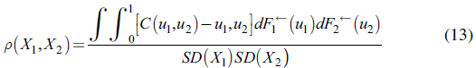
Kendall correlation is given by:
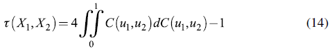
It is observed that the т Kendall is functioning with copulas X1 and X2 while the coefficient of Pearson's lineal correlation only depends on the marginal.
For the copulas analysed in this work, that is, the elliptical and Archimedean copulas, there is a relation between rank correlations and lineal correlations. This work especially focuses on the relation with the r Kendall. The properties of copulas are summarized below:
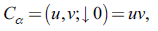
Gumbel Copula

This copula is characterized by having a lower tail dependence and upper tail dependence. Its main properties are:
a) δ = 1 implies
C G = (u, v;l) = uv
the independent copula.
b) As δ → ∞, C Cl (u, v; θ) → min (u,v). This limit is the upper Frèchet-Hoeffding bound. It can be shown that if U and V are two random variables uniformly distributed in (0,1) with copula equal to min (u,v), then IP(U=V)=1
c) Lower Tail Dependence: λ L = 0.
d) Upper Tail Dependence: λ L = 2 -2

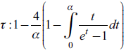
e) Kendall's т :1- -

Clayton Copula

This copula is characterized by upper tail dependence and lower tail independence. Its main properties are
a) θ →0 implies

the independent copula.
b) As θ → ∞, the upper Frèchet-Hoeffding bound is attained
c) Lower Tail Dependence

d) Upper Tail Dependence λ u = 0
e) Kendall's

Frank Copula

This copula is characterized by upper and lower tail independence. Its main properties are:
a) α → 0 implies
the independent copula.
b) As θ →∞, the upper Frechet-Hoeffding bound is attained.
c) Lower Tail Dependence: λ L = 0
d) Upper Tail Dependence: λ v = 0
e) Kendall's
Note that, the Frank copula implies asymptotic tail independence, while the Clayton and Gumbel copulas imply dependence in one of the tails but not in the other. Intuitively, this means that Clayton assigns more probability mass to events in the left tail (joint lower volatility episodes), Gumbel assigns more probability mass to events in the right tail (joint higher volatility episodes), and Frank is symmetric, assigning zero probability to events that are deep in the tails.
It is in this sense that the Clayton and Gumbel copulas describe asymmetric dependence. On the other hand, no clear association in the tails can be observed for the Frank copula.
Student t Copula
This is derived from the t-Student multivariate distribution. It gives a natural generalization of the multivariate t-Student distributions. The t-copula with v degrees of freedom and correlation is written as:ϱ

The t-copula is symmetric and exhibits tail dependence. The coefficient of dependence is:

Where t v+1 is a standard univariate t distribution with v+1 degrees of freedom. Note that two random variables with copula C (u, v; v, ρ ) can be asymptotically tail dependent, even in the extreme case in which they are uncorrelated.
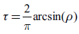
As n →∞ with ϱ ≠0, the normal copula, and therefore, tail independence is obtained. Kendall's tau is related to the correlation coefficient through the formula:
To sum, Table 1 shows parameters estimation.
Table 1 The Elliptical and Archimedean Copulas and Kendall's т
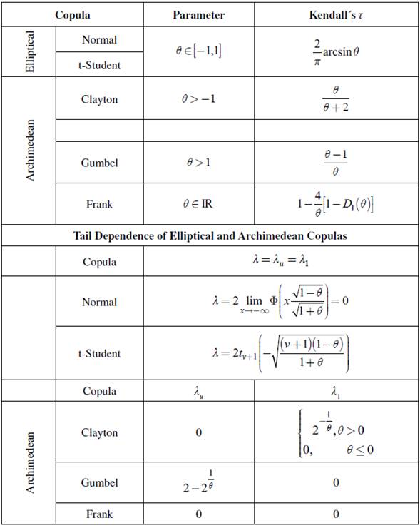
Source: Authors' own elaboration based on Rodríguez (2007) and Fortin and Kuzmics (2002).
EMPIRICAL RESULTS
Basic conditions to estimate GARCH and TARCH models are: stationarity, absence of autocorrelation, and heteroscedasticity in series. The condition of stationarity is checked applying the ADF test. Results reported in Table 2 suggest that the null hypothesis about the presence of unit root is rejected; exchange rate returns are greater than the critical MacKinnon value at a 1 % level. Therefore, it is confirmed that the series are stationary both for levels (logs) and first differences.
Table 2 Augmented Dickey Fuller Test
| Levels | First Differences | |||
|---|---|---|---|---|
| Series | t-Stat | Prob. | t-Stat | Prob |
| Euro | -80.969 | (0.0001) | -29.608 | (0.000) |
| Pound | -76.575 | (0.0001) | -25.614 | (0.000) |
| Peso | -57.974 | (0.0001) | -23.4 | (0.000) |
| Yen | -79.452 | (0.0001) | -27.92 | (0.000) |
Null hypothesis: series have unit root test. * means statistical significance at 1%.
Critical MacKinnon criteria at a significance level of 1% is -3.44
Source: Authors' own elaboration.
The Breusch-Godfrey test is applied. The null hypothesis requires the residuals to not be serially correlated, the probability value to be is greater than 0.05, and the existence of autocorrelation to be rejected.
Table 3 presents ARCH-LM test results; the null hypothesis is rejected. This means that series present heteroscedasticity. Thus, the series exhibits all the properties that need to be analysed using the GARCH approach.
Table 3 ARCH-LM Test Results
| F-statistic | Probability | |
|---|---|---|
| Euro | 146.8261 | (0.000)* |
| Pound | 295.001 | (0.000) |
| Peso | 317.7619 | (0.000) |
| Yen | 333.5778 | (0.000) |
*Probability values are in brackets
Note: ARCH-LM test is the Lagrange Multiplier used to detect ARCH effect.
Null Hypothesis: series does not present heteroscedasticity; this term is distributed as λ 2 (k).
Source: Authors' own elaboration.
Table 4 presents the results from the GARCH model. The GARCH (1,1) model is selected according to the maximum log likelihood method. Results are robust and consistent; all parameters are positive and statistically significant at 1%. The ARCH-LM test is run to confirm that heteroscedasticity disappears after GARCH model estimation; results are significant at 5%.
Table 4 GARCH Results
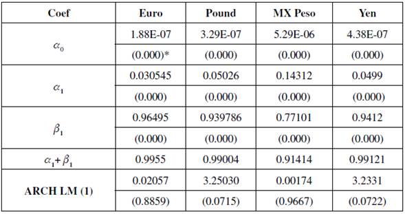
*Probability values are in brackets
Source: Authors' own elaboration.
Source: Authors' own elaboration using estimation results.
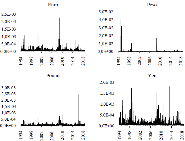
The β 1 coefficient result is, in all cases, higher than a v This implies that there is volatility persistence: in other words, shock effects remain for a long time. α 1 + β 1 is lower than the unit but very close to one. This means that the ARCH process is stationary, so variance does not increase indefinitely. Figure 1 presents conditional volatility estimated by the GARCH (1,1) model.
TARCH Model Results
The GARCH model provides a measurement of symmetric conditional volatility. Financial variables tend to present a leverage effect, which means that volatility is higher when there is an abrupt fall than when a positive shock of the same magnitude occurs. In this sense, GARCH extensions have been developed to capture differentiated effects on variance and asymmetric volatility. This study uses the TARCH to model volatility in exchange rate, and the results are presented in Table 5.
Table 5 TARCH Results
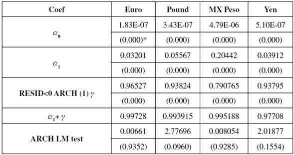
*Values in brackets represent probabilities.
Source: Authors' own elaboration.
The (γ) term represented by RESID<0 ARCH (1) in Table 5 is greater than zero and statistically significant; this condition evidences leverage effect. Positive and negative shocks have differentiated effects on volatility. Good news has an α 1 effect and bad news has α 1 + γ impact: in other words, bad news has a higher impact on volatility than the good news for all the exchange rates analysed. TARCH results suggest that the Euro, followed by the Peso, are the currencies that have highest asymmetry. The ARCH-LM test shows that the model is accurate, probability values are greater than 0.05, which means that ARCH effect disappears after TARCH estimation.
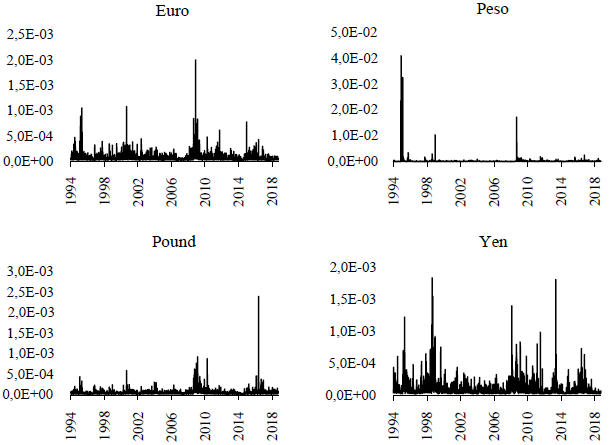
Conditional variance is graphically represented in Figure 2. Results are consistent with the GARCH model. There are common volatility periods as well as some other are individual effects for each currency; for example, in 2013 when Japanese authorities started a quantitative easing programme, or in 2016, when the BREXIT process started (to mention some of the most significant events).
Copula Results
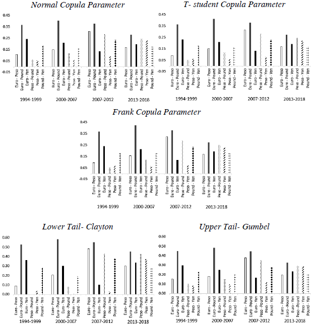
Conditional dependence results are graphically represented in Figures 3 and 4. Empirical evidence signals that, when asymmetry is included in volatility estimation, conditional dependence is higher in most cases. In other words, dependence estimated using TARCH variance is slightly higher than with volatility estimated by GARCH.
Source: Authors' own elaboration with estimation results.
Figure 3 Conditional Dependence (GARCH Model)
Source: Authors' own elaboration with estimation results.
Figure 4 Conditional Dependence (TARCH Model)
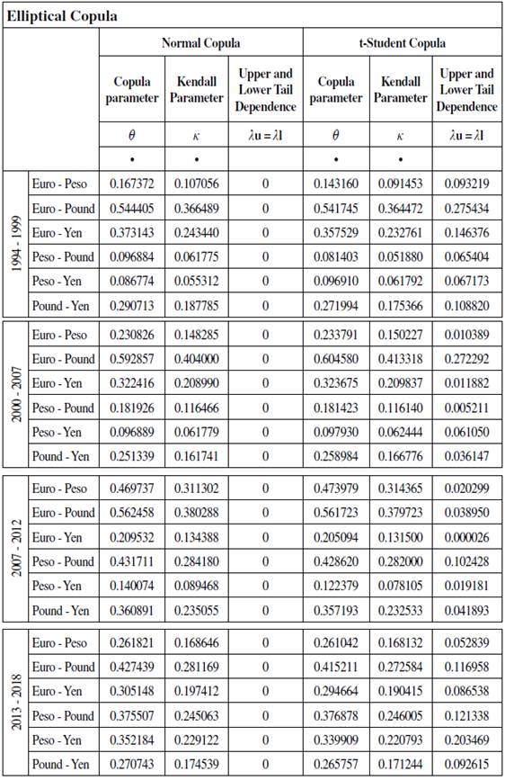
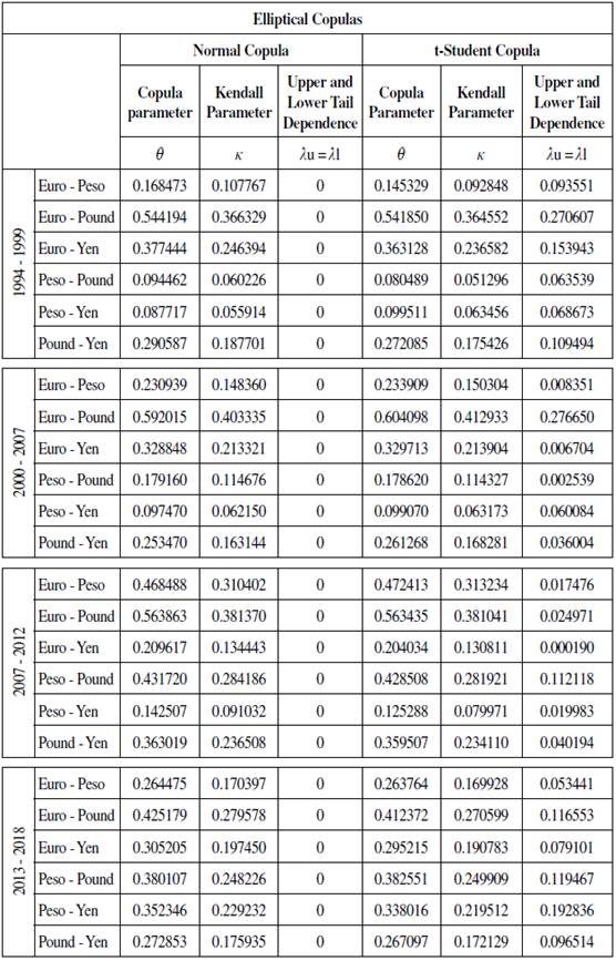
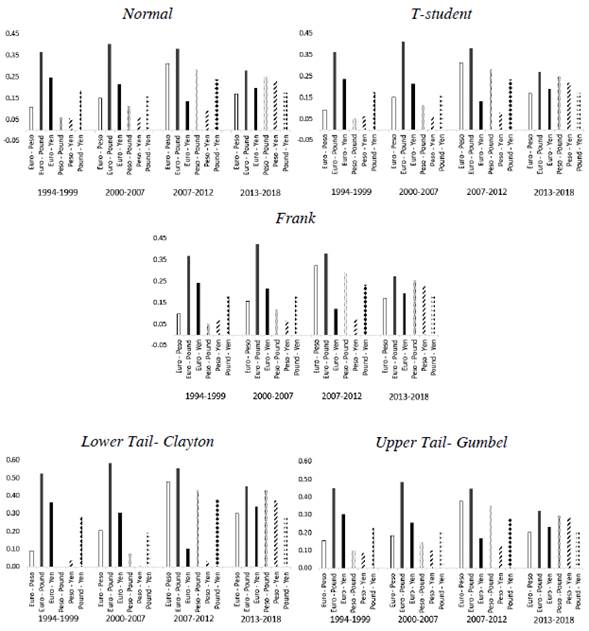
Copula parameters given by Normal, T-student, and Frank Copulas evidence that the Euro and the Pound are the most correlated currencies. Dependence between the Euro and the Pound increased in the periods before the Global Financial Crisis (GFC) and decreased after that moment. The Yen and the Pound presented higher correlation during the periods between (1994-1999) and (2007-2012). This could be related with the impact of the Asian and the GFC crisis.
The Mexican Peso is the only currency that has increased its dependence parameters with the rest of the currencies in the sample from 1994 to 2012; after crisis its relation decreases, except with the Japanese Yen. This can be partly explained due to the Mexican peso being one of the most traded emerging currencies in the world. This currency becomes, therefore, a speculative instrument, vulnerable to other currencies movements.3
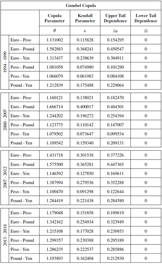
In terms of conditional tail dependence, Clayton and Gumbel Copula evidence that Upper tail dependence is higher than the Lower one. This means that, dependence between currencies does not increase during high volatility periods; correlation is higher during low volatility periods (except for Euro-Peso (1994-1999) and Peso-Pound, Peso-Yen and Pound-Yen (2000-2007). Detailed results are presented in Appendix 1. Results are consistent with those obtained by Fortin and Kuzmics (2002) and Nikoloulopoulos, Joe, and Li (2012).
Some mechanisms behind variations in the exchange rate dependence could include the following: common or differentiated monetary policy responses to changes in key international variables (for example: T-bills rate and oil prices); monetary programmes including Trouble Asset Rescue Program (TARP) and Quantitative Easing (QE), which increased worldwide liquidity; and news that changes investors' expectations motivating global asset allocation.
CONCLUSIONS
This paper has aimed to analyse asymmetric volatility dependence between the British Pound, Japanese Yen, Euro, and Mexican Peso compared to U.S. dollar during different periods of turmoil and subsequent calm sub-periods from 19942018. GARCH and TARCH models were used to model conditional variance. Once conditional volatility is estimated, Copula approach is employed to measure bivariate dependence between exchange rate volatility.
The TARCH model results indicates that there is leverage effect in series, which means that, negative news has a larger impact on the degree of dependence than positive news. Exchange rate series also presents long memory and persistence of shocks in the volatility.
In terms of copula results, the assumption of asymmetrical tail-dependence distribution is sustained. The empirical joint distribution of exchange rate volatility pairs displays high tail-dependence in the lower tail and low tail-dependence in the upper tail.
The copula results show strong evidence of time-varying and high average (tail) dependence in exchange rate volatility by pairs. These results have several important implications for hedging strategies and diversification benefits for FX traders and institutional investors. They also have important implications for both global investment risk management and international asset pricing by taking into account joint tail risk.
In this sense, currencies are assets used to build investment portfolios. Non-linear and extreme correlation level between two series is key information to be able to take financial decisions, in terms of diversification. On the other hand, exchange rate is one of the most important determinants of real return in a financial investment; thus, information about the common behaviour in currencies is also crucial to decide where to invest, according to market conditions (periods of calm and turmoil). Regarding pricing, correlation options or rainbow options are options relating to one asset that are only activated when a second asset moves in or out of a specific range. Extreme dependence is very important in terms of pricing these options and some other financial instruments.
Future research could include analysis of other variables, for example: commodities, bonds, and equities. Other GARCH models could also be included to compare results. In economic terms, future research may analyse fundamental factors to explain mechanisms and implications behind the exchange rate dependence.