María José Pérez-Fructuoso*, Almudena García Pérez**

* Professor of Mathematics, UDIMA, Madrid Open University. E-mail: mariajose.perez@udima.es

** Associate Professor of Financial Mathematics, University of Alcalá de Henares E-mail: almu.garcia@uah.es

RECIBIDO: septiembre 2008 APROBADO: julio 2009

ABSTRACT:

An accurate estimation of extreme claims is fundamental to assess solvency capital requirements (SCR) established by Solvency II. Basing on the Extreme Value Theory (EVT), this paper performs a parametric estimation to fit the motor liability insurance historical datasets of two significant and representative companies operating within the Spanish market to a Generalized Pareto Distribution. We illustrate how EVT improves classical adjustments, as it considers outliers apart from mass risks, what leads to optimize the pricing decision-making and fix a risk transfer position.

KEY WORDS:

Generalized Pareto Distribution, Tail estimation, Solvency II, excesses over high thresholds, Solvency capital requirements, XL Reinsurance, risk measures

RESUMEN:

Una estimación precisa de las reclamaciones extremas es fundamental para evaluar las exigencias de capital de solvencia establecidas por Solvencia II. Basándonos en la Teoría del Valor Extremo (TVE), este artículo realiza una estimación paramétrica para ajustar una distribución de Pareto Generalizada a los datos de seguros de automóvil de dos importantes y representativas compañías de seguros que operan en el Mercado español. Así mismo, demostramos como la TVE mejora los ajustes clásicos, al tratar separadamente los siniestros extremos de los riesgos de masa, lo que lleva a optimizar los procesos de tarificación y a fijar una posición determinada de transferencia del riesgo.

PALABRAS CLAVE:

Distribución de Pareto Generalizada, Estimación de cola, Solvencia II, reclamaciones por encima de un umbral, Exigencias de capital de solvencia, Reaseguro de exceso de pérdidas (XL), Medidas de riesgo.

RÉSUMÉ:

Une estimation précise des réclamations extrêmes est fondamentale pour évaluer les exigences du capital de solvabilité établies par Solvabilité II. Sur base de la Théorie de la Valeur Extrême, cet article réalise une estimation paramétrique pour ajuster une distribution de Pareto Généralisée des données des assurances automobiles de deux compagnies importantes et représentatives d'assurances du Marché espagnol. De même, nous démontrons comment la Théorie de la Valeur Extrême améliore les ajustements classiques, par un traitement séparé des sinistres extrêmes des risques de masse, ce qui optimise les processus de tarification et fixe une position déterminée de transfert de risque.

MOTS-CLEFS:

Distribution de Pareto Généralisée, Estimation de queue, Solvabilité II, Réclamations hors seuil, Exigences du capital de solvabilité, Réassurance de pertes excessives (XL), Mesures de risque.

RESUMO:

Uma estimação precisa das reclamações extremas é fundamental para avaliar as exigências de capital de solvência estabelecidas por Solvência II. Baseando-nos na Teoria do Valor Extremo (TVE), este artigo realiza uma estimação paramétrica para ajustar uma distribuição de Pareto Generalizada aos dados de seguros de automóvel de duas importantes e representativas companhias de seguros que operam no Mercado espanhol. Da mesma forma, demonstramos como a TVE melhora os ajustes clássicos, ao tratar separadamente os sinistros extremos dos riscos de massa, o que leva a otimizar os processos de tarifação e a estabelecer uma posição determinada de transferência do risco.

PALAVRAS CHAVE:

Distribuição de Pareto Generalizada, Estimativa de fila, Solvência II, reclamações acima de um limite, Exigências de capital de solvência, Resseguro de excesso de danos (XL), Medidas de risco.

1. INTRODUCTION

Solvency II, the new global framework of European insurance supervision (IAIS, 2003 and 2005; IAA, 2004), includes the behavior of extreme events among the insurers' overall financial position parameters, by contrast with Solvency I, which did not consider the whole variety of risks (IAIS, 2005, and IAA, 2004).

With extremes being low-frequency, high-severity, heavy-tail-distributed occurrences (Këllezi and Gilli, 2000), the classical risk theory is not entirely explicative. Extremes fluctuate even more than the risks of volatility and uncertainty and this hinders the assessment of loss amounts and capital sums necessary to their coverage.

Management of extreme events requires a special consideration over a sufficiently wide period to accurately gauge their impact and whole effects (Coles, 2001). While up to now the Pareto distribution was commonly employed to modeling the tails of loss severities, adjustments with Extreme Value Theory (EVT)-based distributions significantly improve tail distribution inference and analysis.

EVT provides insurers with a useful tool to manage risks (Embrechts et al., 1997) , for it allows a statistical-based inference of extreme values in either a population or a stochastic process, and hence a more accurate probability estimation of more extreme events than the historical ones. By modeling extremes aside the global sample data, EVT captures high values at the tail (outliers) and situations exceeding the records, not needing to turn to the global distribution of the data observed. Consequently, the study of extreme risk preserves insurers' stability and solvency when facing the occurrence of extreme losses. The application of statistical models helps to more precisely measuring risks and optimally deciding on capital requirements, reserving, pricing and reinsurance layers.

Similarly to McNeil and Saladin (1997), McNeil (1997), Embrechts et al. (1999), Cebrián et al. (2003), or Watts et al. (2006), we illustrate the possibilities of EVT by means of an empirical study on the loss claims databases of two representative insurers operating within the Spanish motor liability insurance market.

We underline the importance of analyzing largest losses, not only for the reinsurer, but also for the direct insurer, to accurately infer the occurrence of extreme events upon historical information. Since uncertainty of major events may be lowered with a limit distribution of extreme claims ascertaining both their probabilities and return periods, extreme-modeling-based inference becomes an additional, valuable input to the information system supporting each insurer's solvency decision-making process (i.e., within the Solvency II framework).

The remainder of the paper is organized as follows. Section 2 summarizes those EVT results underlying our modeling. Section 3 describes the sample databases of two Spanish motor-liability insurers and presents some preliminary results on the historical losses of each company. Section 4 models the extreme events analyzed. Section 5 applies our modeling to approximate the reinsurance's risk premium as well as two significant solvency-linked risk measures: the VaR and the TVaR. Section 6 applies EVT as a management tool. Finally, Section 7 concludes.

2. THEORETICAL BACKGROUND: THE GENERALIZED PARETO DISTRIBUTION AND THE PICKANDS-BALKEMA-DE HAAN THEOREM

Among EVT results, the Generalized Pareto Distribution is a powerful tool to model the behavior of claims over a high threshold, and in particular, to establish how extreme they can be. In close connection, the Pickands-Balkema-De Haan theorem, another important result from EVT, states that the distribution function (df) of excesses over a high threshold may be approximated by the GPD (Beirlant et al., 1996; Kotz and Nadarajah, 2000; Reiss and Thomas, 2001; Embrechts, Klüppelberg and Mikosch, 1997 ; and De Haan and Ferreira, 2006).

Let X_1,n, X_2,n, ..., X_n,n be a sequence of independent random variables with a common continuous distribution, the peaks over a threshold method allows us to infer the distribution of the observed values once they become higher than a threshold u.

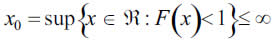
Setting up a certain high threshold u, and being x0 the right endpoint of the distribution:

Then, the function of excesses larger than u is defined as:

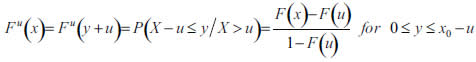
where x represents the observed value (i.e. gross claim loss in our study) and y stands for the excess over the threshold u, i.e. y=x-u.

With the value of the threshold being optimized, it is possible to fit F^u(x) to a Generalized Pareto Distribution (GPD) when u reaches a sufficiently high value:

The GPD is a two parameter distribution with df:

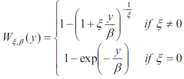
where y≥0 if ξ≥0, and if ξ>0, with ξ and β being the shape and scale parameters. When ξ>0, we have the usual Pareto distribution and the GPD is heavy-tailed, and the higher the parameter the longer the tail. If ξ>0, we have a type II Pareto distribution, whereas ξ=0 gives the exponential distribution.

3. DATABASES AND MODELING HYPOTHESES

Our analysis focuses on two representative Spanish insurers' motor liability portfolios along a ten year-period. The first one counts on a long, renowned business trajectory.

The second exhibits a more recent history, although significantly improved over the last years of the interval. The diverse comparative situation of both companies raises the quality of the sample, since their relatively divergent situation allows a better study of extreme values in two quite differentiated, but at the same time representative, positions of a growing insurance industry like the Spanish. Data of each company have been distorted in order to maintain their respective corporate identities undisclosed.

Two different concepts are assumed as forming the loss amount:

• The cost of settled claims, summing all net payments already made out
• The cost of non settled claims, comprising all net payments already made out, and/or the reserves for the estimated and still pending future payments.

Data have been updated to 2006 values to avoid the effect of inflation.

Tables 1 and 2 display, on an annual basis, each company's number of claims, together with their total and average individual costs in nominal currency units.

Data in Tables 1 and 2 indicate that both insurers lacked of a stable average cost evolution, due mainly to three reasons: the fact that the final cost is integrated by diverse covers, the different settlement periods, and the occurrence of extreme events.

Other indicators are shown in Table 3 and 4 to describe the behavior of the claims. Dividing claims over policies we obtain a measure of the annual claim's frequency.

The insurer A (Table 3) shows a lower frequency, between 14 and 16 percent, and a weighted average frequency of 14.93 percent in the last 9 years. Its position within the Spanish market is solid and deviations from the average are not strong. The history of the insurer B (Table 4), on the other hand, is less consolidated, with a higher weighted average loss frequency (45.13 percent) only over the last four years of the interval. Nevertheless, the claims frequency over the portfolio is decreasing as the number of policies in portfolio grows[1].

These descriptions and the specific features of the samples gave us some clues for the modeling of the extremes in both companies.

4. GPD ADJUSTMENT TO A SAMPLE OF EXTREME CLAIMS WITHIN THE SPANISH MOTOR LIABILITY INSURANCE MARKET

We develop in this section the parametrical modeling of extremes for the insurers under study. These will be the main steps:

1. Choose the optimum threshold to fit the GPD, by means of the empirical mean excess function.
2. Estimate the model parameters according to the heavytailedness of the distribution, with those estimators that minimize the Mean Squared Error (MSE).
3. Check the goodness-of-fit to the underlying distribution with the Quantile-Quantile plot (QQ plot) and some error measures.
4. Infer future extreme events under the estimated conditional model.
5. Calculate the marginal probabilities and determine the unconditional distribution.

Choice of the optimal threshold

Assuming sample data are independent and stationary, the optimal threshold to fit the GPD results from the mean excess function, e(u)=E[X-u ‌ X>u], which is estimated in practice with the empirical mean excess function,

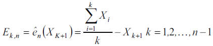
where ê_n(X_k+1) is the mean of the excesses over the threshold u = X_k+1 minus the selected threshold, and k is the ordinal position in the descendent ordered data.

As discussed in Beirlant et al. (1996), data over a certain value of u may reasonably be considered as heavy-tailed if the mean excess plot follows a growing trend. Since the plot is linear with positive gradient, there exists a solid trace that our sample data will fit to a GPD with positive parameter.

At a sufficiently large sampling layer, say 25, the number of excesses of the insurer A is roughly 1,000, with the mean-excess function plotted in figure 1 (left plot).

Figure 1 shows that the function is horizontal between 20 and 70, but straightens out at around 75, what implies that the value of 75 should be taken as the optimal threshold (right plot) for the insurer A dataset, and hence that excesses beyond (as many as 125) might fit to a GPD.

The mean excess function of the 1,000 largest claims covered by insurer B over the ten year period analyzed is sketched in the graphic below:

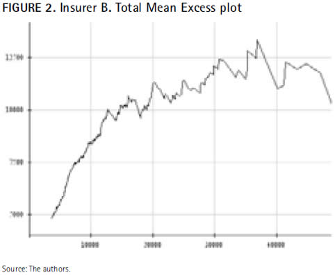
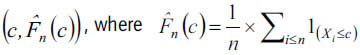
Figure 2 shows the plot of the pairs

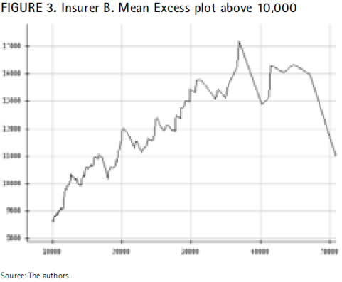
which have an increasing trend from a quite low priority until 30,000 where unexpectedly become plain or even decreasing for the highest thresholds. This means that values beyond 30,000 should not be chosen as the optimal threshold to fit the insurer B dataset to a GPD. At a lower threshold, for instance 10,000, the mean excess plot in Figure 3 exhibits a similar behavior to that observed in Figure 2 (i.e., data describe an increasing trend right up to the highest values).

However, the non growing-linearity of the function for the upper observations, even when the priority is raised, calls into question the suitability of the GPD to fit the insurer B dataset. It is worth then asking whether the sample extreme claims are heavy-tailed or not.

First of all, the QQ plot versus the exponential is useful to address this question, as it permits us to establish both the heavy-tailedness and the fit of the data to a mediumsized distribution like the exponential distribution (McNeil, 1997).

The QQ plot should be expected to form a straight line if the data fit to an exponential distribution. A concave curvature will suggest a heavier-tailed distribution, whereas a convex deviation would indicate, conversely, a shortertailed distribution.

For the insurer A, the exponential QQ plot of excesses over the optimum selected threshold (75) results to be:

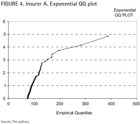
This QQ plot represents the pairs , where empirical Quantiles or rth order statistic X_r,n appear as estimates of the unknown theoretical Quantiles, 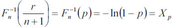, representing the claim levels surpassed in percent of the cases Figure 4 shows that the sample data do not fit to the exponential distribution, since they describe a concave curve rather than a straight line. Concavity, as already stated in general terms, indicates in this specific context that the data distribution is heavier-tailed.

As far as the insurer B is concerned, the exponential QQ plot of the pairs for the percentiles is ploted as follows:

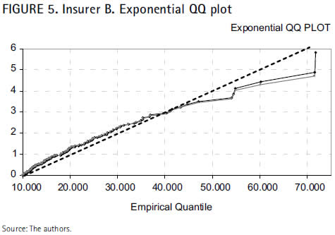
The blue and red lines in Figure 5 represent the respective cloud of points for each percentile, whereas the black line contrasts whether regressions are linear or not.

The slight convex curvature of the adjusting lines with respect to the bisector provides an evident indication that the extreme values of the insurer B cannot properly be captured by the exponential distribution. But the fact that those lines are almost straight leads to think that the largest claims of the insurer B might not be as heavy as those of the insurer A. In such case, the GPD adjusting parameter, although positive, would adopt a value very close to zero.

The outcomes of the QQ plot have been further verified with the likelihood-ratio and the Hasofer-Wang tests, employed by the program XTREMES (Reiss et al., 2001) to measure the data goodness-of-fit to the exponential distribution. Accordingly, the hypothesis of exponential tail (null hypothesis) should be rejected if both tests yield values close to zero, whilst values near 1 shall determine the non-rejection of the null hypothesis, and therefore, the assumption that the tail distribution decreases exponentially.

After the verification was done, p-values of the insurer A tests above the threshold 75 turned out to be 0.00000113 with the likelihood-ratio test, and 0.00000167 with the Hasofer-Wang test. For the insurer B, p-values are 0.09 with the likelihood-ratio test, and 0.145 with the Hasofer- Wang test.

Results of both companies lead to reject the null hypothesis and consequently the exponential distribution as well. Nevertheless, for the insurer B, though p-values approach to zero for observations above 10,000, the tests do not result null, what requires deeper analysis when fitting the parametric distribution.

Parameters estimation

Applying the program XTREMES to fit the insurers A and B sample claims to a GPD, and selecting the Drees-Pickands estimator for the insurer A, since it renders the lowest MSE, we find that the adjustment of its 125 excesses over the optimal threshold (75) yields ξ=0.488146, β=13.0959 and μ=75.1893 as parameter estimates.

The QQ plot reflects the goodness-of-fit between the empirical Quantiles on the x-axis, and the theoretical Quantiles,

on the y-axis, in such a way that the closer the theoretical value (blue line) approximates to the datasample (bisector), the more optimum the adjustment.

The QQ plot indicates an almost complete equivalence between the empirical Quantiles and the GPD theoretical Quantiles. The coefficient of determination (R-square), 0.9845, corroborates that the fitted distribution captures 98.5 percent of all excesses beyond the threshold. The MSE value of 30.94 was the minimum compared to other GPD fittings, thus indicating that the empirical values do not significantly deviate from our theoretical projection. Finally, the Relative Deviations Average (RDA) is virtually null, reaching only 0.0168.

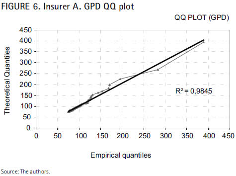
The linearity of the QQ plot, as well as the outcomes of the diagnostic measures, reveal that, in the case of the insurer A, the 125 most severe claims larger than 75 reliably fit to a GPD with parameters ξ=0.488146, β=13.0959 and μ=75.1893.

As to the insurer B, conversely, we applied the XTREMES algorithm to fix the optimal threshold, for although the empirical mean excess function proves to be insufficient, the QQ plot suggests that the extremes will likely fit to a heavy-tailed distribution.

Maximum-likelihood was selected among a variety of estimation methods since it minimizes both the MSE and the RDA. Accordingly, the graphic below displays the estimated parameter for the extremes under discussion:

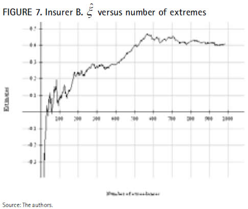
Figure 7 shows that a value around 0.4 is obtained for 500 observation, whereas the parameter becomes negative by maximum-likelihood for less than 50 observations, what implies a short-tailed distribution tending to a right endpoint, in strict coherence with the shift downwards displayed by the mean excess plot, and leads to conclude that the largest observations of the insurer B do not fit to a GPD. And despite the fact that the dispersion of the major values reduces their goodness of fit, we apply the optimal fit rendered by the software XTREMES, i.e. the 159 extreme values over a threshold fixed at 11,908.

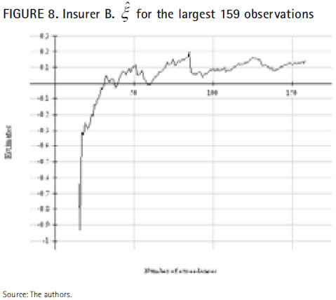
As the next graphic reflects, the tail index ξ estimated by maximum likelihood for those 159 observations remains quite steady at around 0.1.

The mean excess plot of the insurer B at a threshold set at 11,908 shown in figure 9, exhibits a growing trend until approximately 37,000, but stabilizes and even decreases beyond.

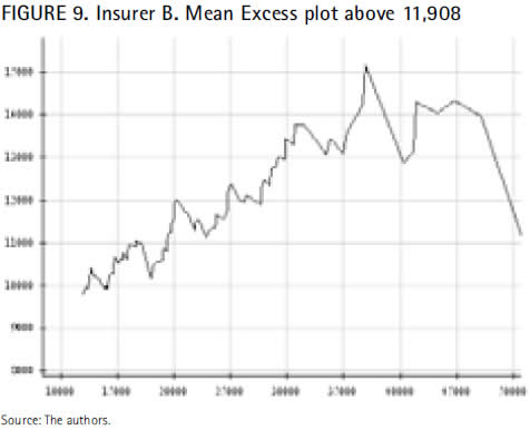
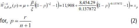
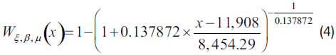
One may wonder if this non-increasing pattern at the tail is relevant enough to cast into doubt the adjustment of the estimated GPD to the claims of the insurer B over 11,908, whose parameters are ξ=0.137872 β=8,454.29 and μ=11,908.

It is necessary, then, to check the GPD QQ plot, with the estimated theoretical Quantiles resulting from:

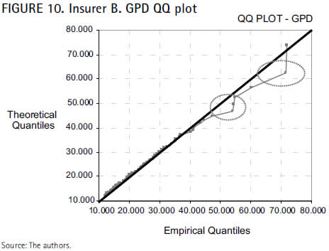
For two similar series of claims (71,851 and 71,541; 54,792 and 54,420, respectively), the mean excess plot decreases at the tail, what at the same time increases the goodness measures (up to MSE = 1,274.388 and RDA = 0.0171) and does not reduce effectiveness, for R² is still of an accurate 99.32 percent. Moreover, disregarding the last observations, R² raises to 99.8 percent, while the goodness measures significantly decrease (MSE = 194,556 and RDA = 0.01469), as displayed in the next QQ plot.

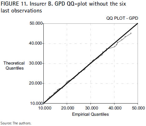
Considering the linearity of the QQ plot and the outcomes of both MSE and RDA, the goodness-of-fit of the estimated GPD to the extremes of the insurer B seems entirely reliable.

Goodness-of-fit

Based on the previous parameters estimation, the GPD function of the insurer A is given by

.

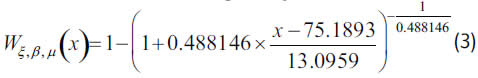
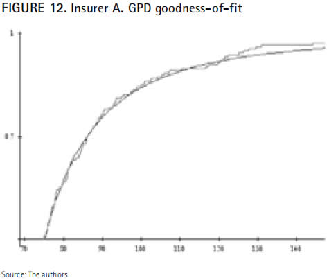
The plot shows a virtual coincidence between both distributions, what suggests an accurate capture of the claims exceeding the optimal threshold (75). Nevertheless, it seems that the theoretical distribution (black line) at the tail shows values slightly lower than those of the empirical ones (red line). Future claims will lead us to a more accurate adjustment.

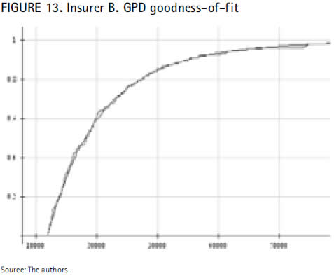
With respect to the insurer B, the graph below reflects that claims larger than the optimal threshold (11,908) perfectly fit to the previously calculated GPD:

Conditional inference and prediction

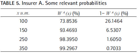
Some relevant solvency-based probabilities are calculated in this Section, on the basis of both the estimated GP df and the estimated GP survival function.

As far as the insurer A is concerned, we find that, say, 99 out of the next 100 claims over the threshold will cost less than 350, whilst the other 1 will cost more:

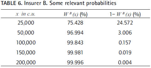
Our finding for the insurer B is that, say, 970 out of the next 1,000 claims exceeding the layer fixed at 11,908 remain under 50,000.

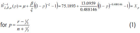
The inverse of the insurer A probability function generates the estimated theoretical Quantile function (equation (1)) that makes it possible to perform the following relevant calculations in terms of solvency,

resulting that, for instance, an excess of 75 with probability 99 percent will not cost more than 302.387, while 1 out of 100 claims over the threshold will probably surpass the reference value of 302.387.

Applying the equation (2) to the insurer B, we find that excesses over a threshold set at 11,908 will cost less than 66,291, with a probability of 99 percent. This means that 100 claims over the threshold will have to occur to find one larger than 66,291 c. u.

Solvency Unconditional inference and prediction

By properly approximating the conditional probabilities and Quantiles as done before, insurers will be able to estimate the unconditional ones and take optimal decisions on free funds, solvency margins and reinsurance cession.

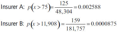
The probability p' of an extreme over an amount (X) happening results by multiplying the GPD-adjusted conditional probability of claims over a certain threshold, but can also be obtained as the ratio between the number of events (insurer A: 125; insurer B: 159) over the threshold (insurer A: 75; insurer B: 11,908) and the total claims occurred in the respective portfolios over the ten year period (insurer A: 48,304; insurer B: 181,757):

At this stage, a key question to determine the capital requirements lies in calculating the expected number of claims over a certain threshold over the next year. This issue may be solved by extrapolating onto the next year either the historical number of claims or the historical loss occurrence frequency per policies, or even by assuming a Poisson distribution.

The claim frequency per policy was very stable in the case of the insurer A. It remained within a short range of between 13 and 16 percent over the last nine years, (shown in y-axis right in figure 14).

and has gradually decreased, in the case of the insurer B, due to the strong growth of its portfolio over the last four years, finally stabilized at levels around 40 percent (y-axis right in figure 15).

Past tendencies of the insurer B, however, will not probably be extrapolable to the close future and the recent behavior will more likely be explicative of the following years.

If we take the historical claim's number of the insurer A (insurer B) to infer forthcoming frequencies, what was done by means of a linear adjustment with R² = 95.93 percent (R² = 99.55 percent for the last five years), we find that:

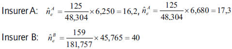
Between 6,250 and 6,680 (45,765) claims are expected to occur as a global number and 16 or perhaps 17 (40) out of them are expected to exceed the threshold u set at 75 (11,908). So, being û_e the expected number of large claims higher than u:

Alternatively, if we extrapolate the portfolio and the claim frequency per policy (red line in figures 16 and 17) of the insurer A (insurer B), with linear adjustment R² = 98.9 percent (R² = 99.67 percent, considering only the last five years), and apply it to the weighted mean claim frequency ("weighted" mean the loss frequency of the last five years), the expected total number of claims reaches as much as 6,390 (51,071).

This number remains, as regards the insurer A, within the interval previously established, even for the largest claims , whilst the estimation is slightly more pessimistic for the insurer B, since its expected claim frequency over the next year will probably be lower than the average of the last five years .

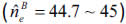Finally, if the choice is to assume a Poisson distribution, its parameter turns out to be for the insurer A.

Selecting this value as the average number of claims is feasible, as the number of claims above the threshold 75 remained stable over the time, and also due to the fact that the mean and variance of the distribution are similar. It would not be valid to assume, by contrast, 15.9 as the average number of claims for the insurer B, since its number of claims exceeding the threshold gradually increased over the years, and the variance of the distribution stands quite above the mean.

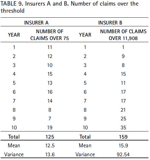
With respect to the insurer A, and assuming a Poisson distribution, one may expect as much as 18 claims exceeding the threshold (fixed at 75) over the next year, with a 95 percent level of confidence P_12.5(n=18) = 0.948. Such approximation renders a more slightly pessimistic projection. For this reason, and according to the principle of prudence, 18 will be assumed as the expected number of claims larger than 75.

Then, extremes larger than 75 expected to exceed a loss amount of, say, 350, over the next year can be quantified as follows:

As far as the insurer B is concerned, a conservative approach suggests that the number of claims larger than 11,908 fits to a Poisson distribution if, and only if, is taken as the highest number of claims among those observed over the ten year interval (that is, 35). Under such assumption, the expected number of claims above 11,908 will equal 45, with a notable 95.75 percent level of confidence.

Since this approximation yields very similar results to those obtained by extrapolation based on the number of policies, the principle of prudence leads to assume the latter as the expected number of claims larger than 11,908. Subject to those conditions, extremes over 11,908 expected to exceed 50,000 over the next year will be

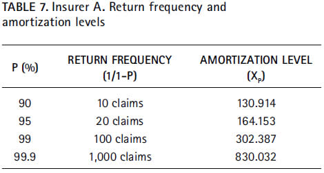
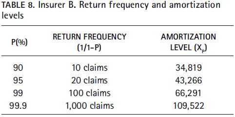
Conversely, and assuming the hypothesis and , it is possible to use equations (1) and (2) to calculate the expected loss amount X, given a certain return period.

For the insurer A (insurer B), Table 10 indicates that the amount 1,509 (146,147) will not be exceeded with 0.5 percent (1 percent) probability over the next year, and reflects a return period of 200 (100) years for such kind of claims.

Thus, we find that the expected amount for the 100-year return period of the insurer A is 2.24 times the expected claim for the insurer B for its corresponding 100-year return period. These are the explanatory reasons:

• The threshold of the insurer A is almost twice as much as that of the insurer B.
• The tail index of the insurer A (and therefore its extreme claims-linked probabilities) is larger than the one fitted for the insurer B.

5. APPLICATION TO THE XL REINSURANCE: PARAMETRIC ESTIMATION OF THE NET REINSURANCE PREMIUM

Excess of Loss reinsurance - XL covers a primary insurer against losses over a certain amount, referred to as layer (P). On the basis of its own risk portfolio, the reinsurer must know exactly both the kind of severe losses assumed and their best fitting model, since both factors will determine the reinsurance risk premium, RP_XL= E_R(S).

Whereas E_R(S) has traditionally been estimated in a non parametric way upon the historical total loss, we propose in this Section the use of a parametric EVT model to more accurately perform such calculation.

Under the classical risk theory hypotheses, the expected total loss over a period is given by E_R(S) = E(N) × E_R(X). An unbiased estimator of this average is (Reiss et al., 2001):

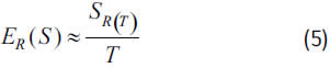
that is, the quotient between the total loss amount occurred along T periods S_(T) and the number T of periods considered.

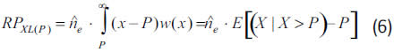
However the reinsurance risk premium can be estimated parametrically:

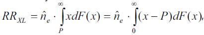
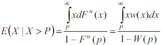
where the number of claims larger than the threshold can be estimated through a Poisson distribution, and the expected loss amount above the layer P, which is covered by the reinsurer, results from the adjusted GPD as follows:

with dF^u(x) = w(x) being the density function of the adjusted GPD.

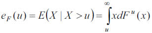
Nevertheless, since the reinsurance layer does not have to coincide with the threshold of the optimized GPD, e_F(u) can be estimated, under the necessary condition P>u, by

It is well known that reinsurers only cover that part of the final cost corresponding to the expected excess over the layer, that is, E [(X ‌ X > P)-P]. Assuming that both the occurrence moments and the loss amounts fulfill the conditions of a compound Poisson process (λ, W), with λ denoting the average claims number over a period, and W the GPD df of excesses above the layer P, the risk premium appropriate to the subsequent period is

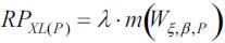
where m(W_ξ,β,P) stands for the expected value of the GPD, with parameters ξ, β, and layer P, such that

For instance, with layers P^A=350 and P^B=50,000 the estimated number of exceeding claims over the next year are, respectively,

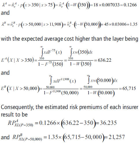
By contrast, a non parametric estimation of the risk premium to be paid by the insurer B (for instance, following the simple equation 7) renders as result 6,675.6, what implies an underestimation of the reinsurer's risk premium.

Even assuming the historical behavior as non significant (since six claims larger than 50,000 took place over the last four years), and applying the average cost times the number of expected excesses

the net premium would be 29.2 percent lower than that estimated with parametric methods.

This leads to the logical conclusion that non-parametric methods should not be applied when the historical background available is insufficient, which is precisely the case of the insurer A, with only one historic claim larger than 350.

The adjustment of data on severe losses with EVT not only appears relevant for the reinsurer. Knowledge on its own extremes allows the direct insurer to optimally decide two key questions: (a) either reinsuring the risk of losses over a certain layer in exchange of a premium, or retaining a sufficient financial capacity to accept claims over a certain loss layer, (b) choosing the suitable thresholds for both cession and retention.

6. EVT AS A MANAGEMENT TOOL

In the light of the imminent implementation of Solvency II, insurers are developing growing efforts to determine their optimal capital level, considering that a higher cession to reinsurance (i.e. low priorities) involves a lower level of free funds (less remuneration of the net worth), but also a larger cost to cover severe risks, and vice versa.

Under Solvency II, capital requirements (Solvency Capital Requirement, SCR) will be statistically-based and suitable to be determined through measures relying on both cost distributions and risk percentiles (Dowd and Blake, 2006), such as VaR and TVaR, which can be approximated by the GPD distribution fitted as well.

These are the conditioned VaR and the TVaR with the adjustment of the GPD for a threshold optimized, respectively, at 75 (insurer A) and 11,908 (insurer B):

7. CONCLUDING REMARKS

Insurers and reinsurers share a deep concern in accurately estimating the probability of claims over a certain threshold. Expertise in handling extreme risks is decisive to determine that level of financial capacity required to assuming or ceding extreme losses.

Our analysis of sample data from insurers operating within the Spanish motor liability insurance market illustrates that fitting a GPD to claims above a high threshold is a powerful tool to model the tail of severe losses.

Classical approaches are good at modeling mass risks, but not so much at capturing rare or extreme risks escaping from the domain of attraction of the traditional distributions. Conversely, EVT has nothing to do with mass risk, but renders a good performance when it comes to modeling rare or extreme losses.

Not intending to overestimate the predictive properties of EVT, but rather complement the traditional methods, we show that a sole cost distribution cannot suitably model a portfolio as a whole. Extreme losses require independent modeling with self-specific distributions, so that the adjustment of classical models to blunted losses is more efficient and less biased, and the fitting of extreme values to the peaks refine the ultimate inference wished by any insurer.

Whereas the classical risk theory appropriately determines capital level for a certain probability of ruin, EVT does the same with regard to the volume of funds necessary to attend peak claims.

Being familiar with the behavior of extreme events allows the insurer to decide either assuming or ceding them and, as required by Solvency II, determine risk measures (such as VaR or TVaR). At the same time, it permits the reinsurer to asses the expectation of losses over a certain layer, and hence the risk premium to perceive in exchange. As we have illustrated in this paper, insurers must choose the best option available in terms of cost of capital. That is, either keeping a financial capacity to cover VaR or TVaR, or paying an XL reinsurance premium.

FOOTNOTES

[1] The decreasing trend in the claim frequency has several reasons: better underwriting rules, more restricted products and the portfolio cleansing.

REFERENCES

Beirlant, J., Teugels, J. L. & Vynckier, P. (1996). Practical Analysis of Extreme Values. Leuven: Leuven University Press.         [ Links ]

Cebrián, A. C., Denuit, M. & Lambert, P. (2003). Generalized Pareto fit to the society of actuaries' large claims databas. North American Actuarial Journal, 7(3), 18-36.         [ Links ]

Coles, S. (2001). An introduction to Statistical Modeling of Extreme Values. London: Springer.         [ Links ]

De Haan, L. & Ferreira, A. (2006). Extreme value theory: An introduction. New York: Springer Series in Operations Research and Financial Engineering.         [ Links ]

Dowd, K. & Blake, D. (2006). After VaR: the theory, estimation and insurance applications of quantile-based risk measures. The Journal of Risk and Insurance, 73(2), 193-229.         [ Links ]

Embrechts, P., Resnick, S. I. & Samorodnitsky, G. (1999). Extreme Value Theory as a Risk management Tool. North American Actuarial Journal, 3(2), 30-41.         [ Links ]

Embrechts, P., Klüppelberg, C. & Mikosch, T. (1997). Modelling extremal events for Insurance and Finance. Applications of Mathematics. Berlin: Springer.         [ Links ]

International Actuarial Association (IAA) (2004). A global framework for insurance solvency assessment. Research Report of the Insurance solvency assessment working party. Available at http://www.actuaries.org/LIBRARY/papers/global_framework_insurer_solvency_assessment-public.pdf, http://www.iaisweb.org/__temp/Insurance_core_principles_and_methodology.pdf        [ Links ]

International Association of Insurance Supervisors (IAIS) (2005). A new framework for insurance supervision: Towards a common structure and common Standards for the assessment of insurer solvency. Available at http://www.iaisweb.org/__temp/Framework_fir_insurance_supervision.pdf        [ Links ]

Këllezi, E. & Gilli, M. (2000). Extreme Value Theory for Tail-Related Risk Measures. Netherlands: Kluwer Academic Publishers.         [ Links ]

Kotz, S. & Nadarajah, S. (2000). Extreme value distributions. Theory and Applications. London: Imperial College Press.         [ Links ]

McNeil, A. J. (1997). Estimating the tails of loss severity distributions using Extreme Value Theory. Astin Bulletin, 27(1), 117-137.         [ Links ]

McNeil, A. J. & Saladin, T. (1997). The Peaks over Thresholds Method for Estimating High Quantiles of loss Distributions, Proceedings of 28th International ASTIN Colloquium. Available at http://www.math.ethz.ch/~mcneil/pub_list.html        [ Links ]

Reiss, R. D. & Thomas, M. (2001). Statistical Analysis of Extreme Values (with applications to insurance, finance, hydrology and other fields). Basel: Birkhäuser Verlarg.         [ Links ]

Watts, K. A., Dupuis, D. J. & Jones, B. L. (2006). An extreme value analysis of advanced age mortality data. North American Actuarial Journal, 10(4), 162-178.         [ Links ]