


 English (pdf)
 Article in xml format
 Article references
 Send this article by e-mail
 Cited by SciELO
  Cited by Google
  Similars in
SciELO
Similars in
SciELO  Similars in Google
 Permalink
1. Introduction
Travel speed is one of the variables to be considered for the correct application of welding. One of the parameters that is affected is the micro-structure of the fusion zone, which was studied in an AA6061 aluminum alloy joined by a laser beam. It was shown that high travel speeds produced V-shaped ripples and a significant amount of heterogeneous nucleation in the axial direction [1]. Another property affected is micro-hardness, where an analysis on laser welded joints for Ti6Al4V titanium alloy exposed that it is higher as the welding speed increases [2]. Another effect found is that the corrosion performance in dissimilar Gas Metal Arc Weld Joints of AISI 304 improves as the speed values are decreased [3]. Study of corrosion is relevant for determining the weld performance since it can be the main cause of failure in some applications [4]. As for the weld bead parameters, a reduction in bead width, bead height and penetration was found when the speed of SS409L Gas Metal Arc Welding is increased [5].
Experimental tests are expensive and time consuming [6, 7], so computational modeling can be chosen for considering the effects of welding. It can be performed by two different approaches, analytical and numerical. The analytical approach is usually performed using the Rosenthal equation, however, this method induces some errors in the results since thermal losses and latent heat are neglected [8]. This equation is opposed to the energy release that can be dissipated by conductive, convective and radiation models, as well as under distortion and deformation scenarios presented in the volumetric internal heat generation rate variable [9]. This expression can be seen in equation 1.
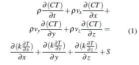
Where:
k: Thermal conductivity [J/mm s C].
T: Temperature in the weld [C].
ρ: Density of the metal [g/mm3].
C: Specific heat of the material [J/g C].
t: Time [sec].
v x : Velocity component in the x direction [mm/sec].
x: Coordinate in the direction of the weld [mm].
• v y : Velocity component in the y-direction [mm/sec].
y: Coordinate in the direction transverse to the weld [mm].
• v z : Velocity component in the z-direction [mm/sec].
z: Coordinate in the direction normal to the weld surface [mm].
S: Volumetric internal heat generation rate [J/mm 3 sec].
On the contrary, numerical methods do take these thermal losses into account, so they are preferred when there is a high energy input [10]. Numerical simulations can be run by pure conduction or can include fluid flow. When the latter is employed, it has been shown that heat affected zones are narrower and pool depths area greater [11]. In addition, the finite element method [12] or the finite volume method can be used [13]. One of the computer programs that has proven to be useful is ANSYS, which can run simulations that allow coupling thermal and mechanical effects [14, 15, 16].
The effects of travel speed have been evaluated using numerical methods, and different studies have found similar results to the experimental ones. For example, some investigations have determined that increasing the travel speed will cause the maximum temperature to decrease [17, 18]. In addition, the temperature distribution obtained from simulations can be used to calculate phase transformations [19].
In this work, the effect of welding travel speed on the temperature distribution was studied. The methodology implemented was by the finite element method and the ANSYS software. In this case, ASTM A36 structural steel was chosen because it is widely used in industry. For heat input, data were obtained from industrial suppliers. The selected joint was of the butt type since it is versatile and one of the simplest to be applied.
2 Materials and methods
This section contains the methodology performed to set up the simulations, consisting of the geometry, the implemented mesh, the boundary conditions, and the material properties needed to solve the problem.
2.1 Geometry
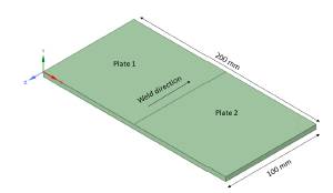
The model employed to run the simulations is illustrated in Figure 1. It consisted of two plates placed end-to-end, since this study was developed for butt welding. The center line is where the arc heat input was applied. The thickness of each plate is 4.5 millimeters.
2.2 Mesh
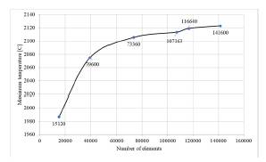
Mesh was selected using a mesh independence study. Overall, six different meshes were evaluated and for each one the maximum temperature was measured. Figure 2 illustrates the variation of the maximum temperature as the number of elements increases. From the figure, it can be determined that from 116640 elements the temperature variation is negligible, so this mesh was selected for the simulations.
The mesh employed to perform the simulations is shown in Figure 3. It has 116640 elements and 133497 nodes. In the central line, where the two plates are joined, the density of elements was increased since there is a high temperature gradient. The mesh was created as structured, this means that the discretization error induced by low quality elements is minimal.
2.3 Boundary conditions
Two boundary conditions were applied. The first consisted of convective heat transfer from the surfaces to the surrounding air, which was imported from the ANSYS library. The second was the energy input, where the parameters employed for its calculation are listed in Table 1. The chosen travel speeds of the applied energy were varied from 120 to 300 [mm/min]. All values related to arc welding energy were entered using the moving heat source extension.
3 Results and discussion
The effect of the travel speed was determined by the thermal behavior calculated from the model. The temperature values were obtained from the center point of the bottom face of the plates, since this point is on the face opposite to the one where the heat input is applied. Therefore, if the fusion point is reached there, full penetration will be guaranteed.
Figure 4 illustrates the temperature variation in the first 50 seconds for each velocity. From the different curves, it can be observed that the peak temperature decreases while the welding travel speed increases, this occurred due to the shorter time exposed to heat input. Additionally, the travel speeds equal to 135 [mm/min] and 120 [mm/min] were the only ones that exceeded the fusion point of ASTM A36 Structural
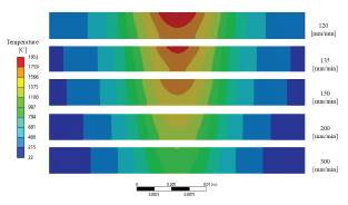
Likewise, the temperature contours were analyzed at the time when the maximum temperature value was reached. Figure 5 shows the five contours obtained for each travel speed at that point. In this case it can also be concluded that the speeds that allow complete melting through the plate were 135 [mm/min] and 120 [mm/min]. However, the speed that would be defined as optimum would be 120 [mm/min], since this has a smaller heat affected zone.
4 Conclusion
The modeling of the thermal behavior when an electric arc welding process is applied was simulated using ANSYS software. It was possible to simulate the temperature variation in the center of the bottom face of the geometry. When the travel speed was 300 [mm/min] the maximum temperature reached was 1043.3 [C] and when it was decreased to 120 [mm/min] the maximum value calculated was 1690.7 [C]. Because of this, it was conceivable to conclude that the increase in the travel speed causes a decrease in the maximum temperature. This must be considered, since in order to properly weld the two plates, the melting point must be exceeded on both the upper and lower faces.
The temperature contours of the different velocities were compared. It could be determined that of the velocities that managed to exceed the melting point, 120 and 135 [mm/min], the one with the lowest value is the optimum. This is because continuing to increase the speed would only enlarge the heat-affected zone.
This work demonstrated the usefulness of computational methods in the study of thermal effects when welding is applied. In this case, the travel speed was evaluated, however, it is also possible to study more variables such as the geometry or the applied energy.

