


 Inglés (pdf)
 Articulo en XML
 Referencias del artículo
 Enviar articulo por email
 Citado por SciELO
  Citado por Google
  Similares en
SciELO
Similares en
SciELO  Similares en Google
 Permalink
1 Introduction
Synchronous motors are highly used in electrical power systems because they are an economical means to improve the power factor of the network, generating a reduction in the cost of electrical energy. This characteristic, together with the ability to operate at constant speeds determined by some types of loads, make synchronous motors indispensable for the industry, with applications in different areas such as: Quarries and cement factories to move ball mills or mills. rollers, compressors, and blowing machines such as extractors, fans, turbofan, centrifugal compressors; in sawmills, in paper mills to move refiners, in rubber and plastic industries to power mixers, steel industries, among many more applications [1 - 3].
The stability of a dynamic system is the ability of the system to maintain its equilibrium point against certain external disturbances, in electrical power systems these disturbances are due to abnormal situations in operation such as variations in loads, failures caused by natural factors, among many other factors. The treatment of the stability problem consists of establishing those conditions for which the operation of the system (generators, motors, or capacitors) turns out to be critical, that is, limit conditions; in such a way that stability is defined for any other condition [4 - 6].
The purpose of this document is to analyze in its different aspects, the specific problem of stability in synchronous motor operates, as a device for converting electrical power into mechanical power, since hyperbolicity and stable structure are strongly related, since when there is presence of an eigenvalue with zero real part, the possibility that the system is structurally stable is broken. Thus, through the implementation of the bifurcation theory, it will be in charge of establishing conditions in the parameters of the dynamic system in question for which the system goes from being stable to being unstable. These conditions occur at a specific value of the parameters called the branch point.
2 Theoretical Formalisms
2.1 Lienard Type dynamics model
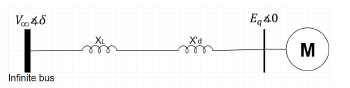
The dynamics of the synchronous motor represented schematically in the Figure 1 is governed by the second order differential equation (1) [7]. The synchronous motor is connected to an infinite voltage bus V i through a reactance xL, and is modeled with an FEM Eq and a transient reactance x' d .
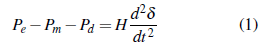
Where δ is the rotor angle of the synchronous motor, H is the constant inertia, P e , P m , and P d are the electrical, mechanical and damping powers respectively, associated with the motor dynamics and defined as:
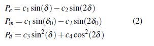
The load P m in the synchronism is assumed constant,
independent of the small variations in speed during external disturbances. Furthermore, the model parameters c1, c2, c3, and c4 are defined by Equation (3) [7] as:
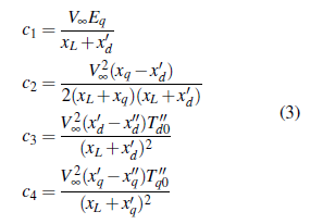
The parameters c1, c2 are the amplitude of the fundamental component and the second harmonic of the electrical power and the parameters c3, c4 decide on the amplitude of the damping power Pd imposed on the rotor of the synchronous motor. The constant damping case can be analyzed when c3
= c4. The steady state equilibrium point of the synchronous motor is given by δ
=
δ
0
and δ
= 0 [7 - 10]. If we define the state variables x1
=
δ
(t) and x2
=
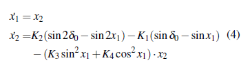
Being Ki
=
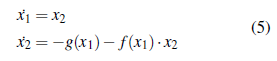
resulting from the second-order differential equation x" + f (x)x' + g(x) = 0. This type of system has the characteristic of presenting limit cycles if the functions f (x) and g(x) meet certain conditions, which are stated in the following Lienard theorem.
2.2 Lienard's theorem
The system f (x,µ) = 0, has a single stable limit cycle around the origin if the functions f (x) and g(x) satisfy the following conditions:
● f (x) and g(x) must be continuously differentiable for every value of x.
● g(- x) = - g(x) for all x, that is, it must be an odd function.
● g(x) > 0 for all x > 0.
● f( - x) = f( x) for all x.
● The odd function F(x) =
2.3 Foundation of nonlinerar dynamics systems
The mathematical model of a dynamic system can be represented in state space by a set of first-order differential equations as observed in Equation (6) [11]:
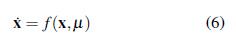
where x e
2.4 Equilibrium points
The equilibrium points for the system represented by Equation (6) are given by
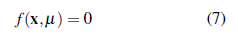
For a given value of /, the solution of Equation (7) will be an equilibrium point for the system given by Equation (6). Once the equilibrium points have been defined, it is necessary to study the classification of their stability through linearization around them, as shown.
Taking xo y µ0 as equilibrium points, the system gyven by Equation (6) can be rewritten as Equation (8) [11]:
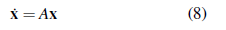
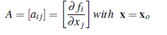
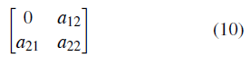
where A is the Jacobian matrix of the system represented by Equation (1), defined according to Equation (9) [11]:
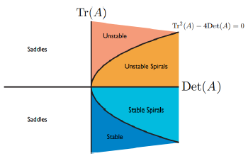
The stability of each of the equilibrium points of the system represented by Equation (6) will depend on the eigenvalues of matrix A; They can also be classified depending on the values taken by the trace of matrix A(Tr(A)) and its determinant (Det(A)). A summary of this is graphically shown in Figure 2 [12,13].
2.5 Hyperbolicity and structural stability
One of the most relevant properties that can be obtained from the eigenvalues of matrix A to characterize the equilibrium point analyzed is the concept of hyperbolicity. If none of the eigenvalues of matrix A has a real part zero, the point x0 is said to be a hyperbolic point. Two consequences of a hyperbolic equilibrium point are the following:
If matrix A has no zero eigenvalues, then x0 is a simple transverse zero of (7). Therefore, by the implicit function theorem, the existence of a smooth function x(µ) with x(µ 0) = x0 that shows the variation of x0 when the parameter / is varied is guaranteed. Furthermore, there is no variation in the number of equilibrium points when µ = µ 0.
The qualitative structure of the phase diagram for the non-linear system is the same as that of the linearized system, this as a consequence of the Hartman-Grodman theorem [14, 15]. This fact is very important from the qualitative characterization of a non-linear system through its linearization. It should be noted that, for non-hyperbolic equilibrium points, the analysis of their stability will not be the same for both systems, that is, it is not possible to conclude about their stability through the criterion of eigenvalues and it is necessary to study by other techniques such as the construction of energy functions [16, 17].
A system can be robust if when making small modifications of a parameter, the trajectories of the phase space are only slightly disturbed, if this is the case, the system is said to be structurally stable. Both concepts of hyperbolicity and stable structure are strongly related since when there is the presence of an eigenvalue with zero real part, the possibility that the system is structurally stable is broken.
2.6 Bifurcation Theory
Bifurcation theory is a branch of applied mathematics where its main interest is the analysis of the Equation (7), where x is an equilibrium solution and / is a scalar parameter, that is, determining how is the variation of x(µ) for when µ varies. The parameter µ is called the branch parameter. A bifurcation point is one where there is a branching or change of the solution. System stability is closely related to this bifurcation phenomenon [18].
2.7 Hopf bifurcation
The Hopf bifurcation is also known as the Poincaré-Hopf-Andronov bifurcation, it is characterized mainly by the appearance or disappearance of a periodic solution (limit cycle) of an equilibrium when the µ parameter of the system represented by Equation (6) causes the eigenvalues to cross the axis imaginary from left to right. There are two types of Hopf bifurcation, supercritical or subcritical, stable, or unstable within a manifold, respectively.
2.8 Hopf theorem
Taking the following considerations for the system described in Equation (6):
The system has an equilibrium point at P0 = (Xo, µo)
The Jacobian matrix of (6) has a conjugate pair of eigenvalues λ = α ± jω such that for a critical value of the bifurcation parameter µ = µ c it holds that α (µ c) = 0, α' (µ c) = 0 and ω(µ c) # 0 where α' =
Except for ± jω (µc) the eigenvalues of the system have a negative real part.
If these conditions are fulfilled, then for a disturbance in the state xi, the dynamics of the system represented by Equation (6) has a stationary solution. The dynamics of the system corresponding to the stationary solution will be stable for μc−μ > 0 and unstable for μc−μ < 0 if α′(μc) > 0. Stable for μc−μ <0 and unstable for μc−μ >0 if α′(μc)<0. For μ = μc the system will have oscillations with period 2π/ω(μc) [19].
3 Simulation and results
For the results obtained in this section, the following values of the parameters were used:
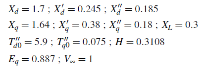
The equilibrium points of the system represented by Equation (4) are given by the Equation (10):
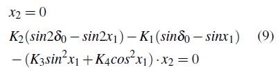
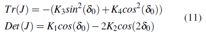
With which the point Pe(δ0, 0) is obtained and its associated Jacobian matrix will be represented by Equation (11):
where α12 = 1, α21 = K1 cos(δ0)−2K2 cos(2δ0) and α22 = −(K3 sin2(δ0)+K4 cos2(δ0)). Therefore, the trace and determinant will be defined as:
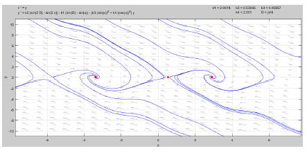
For the parameters of the previous table, we have that Tr(J) < 0 and that Det (J) < 0, with which it is obtained that the equilibrium point of interest is a saddle point as classified in the Figure 3. In addition, two more points are obtained which correspond to sinks, with which the stability of the system will be determined not only by the value of its parameters, but also by the initial conditions taken. By varying the magnitude of the bus voltage to
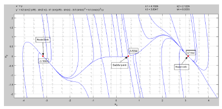
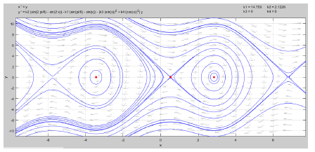
which the synchronous motor is connected, there is a variation in the stability of the equilibrium points, which go from having asymptotic stability to having spiral stability as shown in the Figure 4. When a constant damping value is taken equal to zero, that is K3 = K4 = 0, it is given that the dynamics of the stable points (sinks) become center points, as observed in the Figure 5.
4 Conclusions
Qualitative analysis for nonlinear dynamic systems is of vital importance since in most of these cases the analytical solutions are impossible to determine. Besides, with the bifurcation theory, critical values can be established in the parameters where the stability of the system will present variations. Also, an application of the Hopf bifurcation theorem was presented for the case of an asynchronous motor with variable damping. The conditions that the voltage of the infinite bus to which the network is connected must meet for it to have asymptotic or spiral stability were established. It was determined that when the bus voltage presents variations, the equilibrium points change their dynamics from asymptotic stability to spiral stability. When the synchronous motor enters the instability state, there is only one option for this, and it is the asymptotic type of instability since spiral type instability cannot occur. For the parameters defined in this application, it was observed that Tr(J) < 0 and that Det (J) < 0, that is, the equilibrium point of interest is a saddle point. When a constant damping value is taken equal to zero, this is K3 = K4 = 0, it is given that the dynamics of the stable points (sinks) become center points

