


 English (pdf)
 Article in xml format
 Article references
 Send this article by e-mail
 Cited by SciELO
  Cited by Google
  Similars in
SciELO
Similars in
SciELO  Similars in Google
 Permalink
1 Introduction
Geostatistics plays an important role in applied fields as diverse as ecology [1], agronomy [2], mining [3], meteorology [4], environmental pollution [5], amongst others. Usually, a geostatistical analysis is carried out in three steps, namely: exploratory data analysis, spatial dependence estimation, and kriging prediction [6]. Classical results from decision theory [27] show that under squared loss, the best predictor (BP) is the conditional expectation of the predictor given the information. For normal processes, the BP is equivalent to the best linear predictor (BLP), called simple kriging in geostatistics [8].When the mean is unknown and the random field is normal, ordinary kriging provides as an approximation to the BLP [9]. The solution, in this case, includes an additional constraint to ensure the predictor to be unbiased. Hence, ordinary kriging is a best linear unbiased predictor (BLUP). Such an explicit link between BP and normality calls for testing the normality assumption on the basis of a limited number of observations. The literature has typically relied on univariate normality tests: [10] have studied the spatial distribution of some chemical variables in a mine located in Ireland. The authors use a Kolmogorov-Smirnov test and Box-Cox transformations to achieve normality. [11] study the spatial variability of mechanical resistance to penetration in a ferralsol cropped with corn, in Ilha Solteira, Brazil. The normality hypothesis is tested by using a Lilliefors test. [12] use a SW normality test with data of penetration resistance of soil in a region of Poland. [13] assess the distribution pattern of organic carbon in a region of central Japan. [13] assess distribution pattern of organic carbon in a region of central Japan. They use a SW normality test in a previous step of the analysis. Other references about the use of univariate normality tests with spatially distributed data are [14], [15], [16], [17] and [18]. These are just a few examples on the use of classical normality tests with samples from spatial processes. These tests are defined on the basis of the assumptions of independence and identical distribution. This is clearly inadequate in geostatistics, where the observations are typically spatially correlated. Hence, these tests might be inappropriate to say the least. The literature about normality tests in the presence of spatial correlation is sparse, with the exception of [19], who provide a method for obtaining unbiased estimates of the probability density function by weighting the observations using block kriging, and [20], who use a generalized form of the bootstrap method to model the distribution of the statistic of the Kolmogorov-Smirnov test.
Using classical multivariate normality tests [21, 22] in geostatistics is limited because several samples of the random vector are required. In geostatistics, we generally have only one realization of the random field of interest (just one observation of the process is available). Consequently, such tests (in their usual way) cannot be assumed as a viable alternative under a geostatistical framework. In this work, we focus two aspects on. Initially, we show (through simulation) that using univariate normality tests (SW, SF, AD, etc) in geostatistics is not appropriate because these ones do not take into account the spatial dependence. We also show how the Mahalanobis distance [23] can be adapted to a geostatistical scenario to test for multivariate normality of Y = (Y (x 1 ), ∙∙∙, Y (x n )) T of the random process based on just one an observation y(x) = (y(x 1 ),..., y(x n )) T .
The paper is organized as follows. Section 2 presents an overview of kriging and optimal prediction under normality. In Section 3, we show the approach based on the Mahalanobis distance [23]. A simulation study is developed in Section 4. The paper ends with a short discussion and suggestions for further research.
2 Materials and Methods
In this section we show the basics of simple kriging, ordinary kriging and BP under multivariate normality.
2.1 Simple Kriging and BLP
This section is based on [9], [24], [25], and [26]. Let A be a countable subset of ℝ2. Geostatistics concerns with the analysis of a real valued stochastic process {Y(x): x ∈ A}, which is typically considered to be a partial realization of a stochastic process {Y (x): x ∈ ℝ2}. Let Y = (Y(x1), ···, Y(x n )) T be a random vector following any multivariate distribution Y ~ f (µ, Σ), with µ denoting the mean vector and Σ the covariance matrix. Here T denotes transpose. Assume that 𝔼(Y(x i)) = ß and 𝕍 (Y(x i)) = σ 2 , for all i = 1,..., n. Then Y can be written as
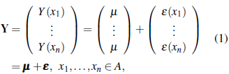
where we assume that
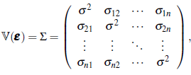
with 𝕍(Y(x i)) = 𝕍(ε(x i)) = σ2,i = 1,··· ,n, and ℂ (Y (x i), Y (x j )) = ℂ(ε (x i), ε (x j )) = σ i,j i,j= 1,..., n, i ≠ j. Suppose we want to predict Y(x0), x0 ∈ A, based on Y where µ and Σ are known. Simple kriging consider linear predictors of the form
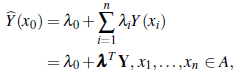
which minimizes the mean-squared prediction error, denoted MSPE, and defined as
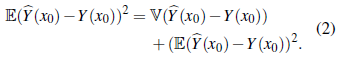
Both terms in Equation (2) are nonnegative and the MSPE will be minimized when each term is as small as possible. The second term in the right hand side of Equation (2) is minimized when
that is, when
On the other hand,

with ℂ(Y, Y(x0)) = (σ10,..., σn0)T = c. Differentiating (3) with respect to λ and equating to zero gives λT = c TΣ-1 . Thus, the BLP is
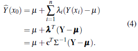
Replacing λT = c TΣ-1 in (3) yields the simple kriging variance
2.2 Ordinary Kriging and BLUP
This section assumes the same conditions as in Section 2.1 but µ is now unknown. The ordinary kriging predictor of Y(x 0) has the same expression as the simple kriging predictor:
Again, the parameters are estimated by minimizing the MSPE as defined in Equation (2). Note that µ unknown implies λ0 to be unknown as well. In this case, we guarantee that 𝔼(
 (x0)) = 𝔼(Y(x0)) by taking λ0 = 0 and
 The predictor is now restricted to these unbiasedness conditions. This is called best linear unbiased predictor (BLUP). The ordinary kriging predictor is consequently defined defined as
and the parameters are estimated by minimizing 𝔼(
(x0) - Y(x0))2 subject to the unbiasedness constraint, that is, by considering the following optimization problem:
To solve (7), we let m denote the Lagrange multiplier. Then, the optimization function is given by min𝕍(
(x0)) + V(Y0) - 2ℂ(
(x0), Y(x0))λi,m
where the second line in the chain of equalities comes from the definition of
, while the third line comes from the fact that covariance is a linear operator [23]. Differentiation with respect to λ and m provides the system

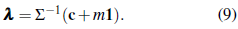
Solving with respect to λ in (8) gives
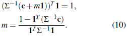
To obtain m, we plug λ into the unbiasedness condition in (8), and find
Plugging (10) into (9) shows that
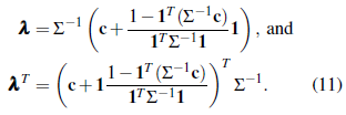
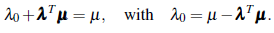
According to the solution in (11), the kriging predictor
(x0) as defined at (6) is given by
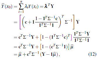
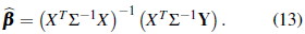
where
 is the generalized least squares estimator of ß defined in Equation (1). From the linear regression model Y = Xβ + ε, with 𝕍(ε ) = Σ, the parameters are estimated by [9]
Taking X = 1 and
 in Equation (13) we obtain,
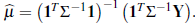 This is the expression for
in Equation (12). The variance of the predictor (12) is given by
This is the expression for
in Equation (12). The variance of the predictor (12) is given by
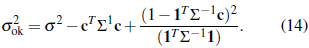
Comparing (5) and (14) we observe that σs 2 k < σs 2 k, since the last term on the right-hand side of (14) is positive. An unknown mean increases the MSPE. In practice, Σ and λ are unknown and must be estimated. Then, a plug-in estimation of Я and m is usually carried out. Thus the ordinary kriging predictor is not a BLUP but an estimated BLUP (EBLUP, throughout).
2.3 Best Prediction
We provide a well know result about optimal prediction, establishing that under the squared loss function, the BP is the conditional expectation of the predictor given the information. For a formal proof the reader is refereed to [25] and [27].
Theorem 2.1. Lef Y = (Y
1,...,Y
n)
T
be a vector composed of afinife collection of n random variables. Denote ihe corresponding realizations as y = (y1,...,yn)T. Lei Y0 be a random variable, and
 = φ (Y) be any fwnciion of Y for φ : ℝn → ℝ. Then, 𝔼[(Y0 -
 )2] affains ifs minimum value when
= 𝔼(Y0|Y).
)2] affains ifs minimum value when
= 𝔼(Y0|Y).
Let {Y (x): x ∈ R 2} be a normal random field [24]. Then
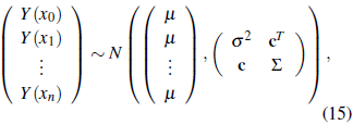
with the vector c and the matrix Σ as defined in Section2.1. Standardproperties ofthemultivariate normal distribution [23] show that, if
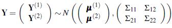
then

 [23]. This property in concert with Equation (15) shows that

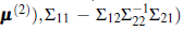
Consequently, the BP under the squared loss function with the stationary normal model is

with variance
The predictors in Equations (4) and (16) are actually the same. Thus, simple kriging is an optimal predictor if the random field is normal. This result has become popular in applied geostatistics ([14], [12], [17], [18]). However, it has been sometimes misunderstood. Some comments are in order:
Data recorded in geostatistics correspond to a realization of a stochastic process. These should not be regarded as one sample of a random variable. Then, testing for univariate normality in this field is meaningless. If {Y(x): x ∈ R 2} is a normal spatial random process then the random vector Y = (Y(x1),..., Y(xn))T ∼ N( µ, Σ). Only when the process is stationary and uncorrelated (mean and variance being constant and Σ = σ2 I) it has sense testing for univariate normality.
Simple kriging, as defined in Section 2.1, is a BP whether the stochastic process of interest is normal, and it is a BLP regardless of whether the process is normal. In practice, using simple kriging is limited because ß and Г are unknown.
Ordinary kriging is not a BP, even when the stochastic process is normal. This predictor is always a BLUP (when µ is estimated and Σ is known) or an EBLUP (when µ and Σ are estimated).
When the stochastic process is normal, maximum likelihood can be used for estimating µ, Σ, and c and consequently for carrying out prediction by using ordinary kriging.
Although common practice, the use of classic univariate normality tests does not make sense in geostatistics. It is required to take into account the spatial dependency structure. The following section proposes an adaptation of the Mahalanobis statistic for this purpose.
3 A New Test for Normality in Geostatistics Based on the Mahalanobis Distance
We now illustrate how a normality test based on the Mahalanobis distance [23], can be adapted to a geostatistical framework. Let A = {x1,..., xn} and Y ∼ N(µ,Σ). It can be shown that

where X 2(n) denotes the central X 2 distribution with n degrees of freedom [28].
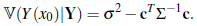
Assume that we have a random sample Y1 , . . . , Yr from the n-dimensional random vector Y, that is we have a random matrix defined as
where Y i j , i = 1 , . . . , r, is a random sample of size r from the random variable Y j , j= 1 , . . . , n. It is known that asymptotically

where
 is the sample mean vector and
 is the sample covariance matrix [28].
Let Y = (Y(x1),..., Y(xn)) T be a realization of size n from a stationary random process {Y(x) : x ∈ R 2} with 𝔼(Y) = µ and 𝕍(Y) = Σ. Suppose we have an observation y = (y(x1),...,y(xn)) T of this process and we want to test the hypothesis

Given µ and Σ known (an unrealistic scenario), the statistic in Equation (17) is calculated as
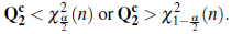
The null hypothesis of normality is then rejected at level α if
On the other hand, let ӯ = (ӯ,..., ӯ)
T
nx1 be a mean vector with ӯ =
 and
and
be the estimated covariance matrix, where
 = Ĉ( Y(x
i
), Y(x
j
)), i, j = 1,..., n. The elements of this matrix can be obtained by fitting to the experimental covariogram a covariance model (Exponential, Gaussian, spherical, etc) through ordinary or weighted least squares [26]. Then, based on ӯ and
= Ĉ( Y(x
i
), Y(x
j
)), i, j = 1,..., n. The elements of this matrix can be obtained by fitting to the experimental covariogram a covariance model (Exponential, Gaussian, spherical, etc) through ordinary or weighted least squares [26]. Then, based on ӯ and
 , we can calculate the statistic defined in Equation (18) as
Consequently, the null hypothesis of normality of the random process is rejected at level a if
We study through Monte Carlo simulation the performance of some classical normality tests (SW, SF, and AD) as well as the tests based on the Mahalanobis distance. The goal is two-fold: to show that using univariate normality tests in a geostatistical context can be inappropriate, and to assess the behavior of the statistics Q1 and Q2 defined in Equations (17) and (18).
4 Simulation Study
4.1 Simulation Under Normality
We simulate normal random fields over regular grids with n = 25,49 and 100 points on a square of 10 x 10 units (Figure 1). Also in order to establish the effect of the spatial distribution of the sampling points on the tests a size n = 100 clustered configuration is considered (Figure 1).
Figure 1 Spatial configurations used in the simulations. Regular grids size n = 25 (top), n = 49 (second panel) and n = 100 (third panel). Clustered grid n = 100 (bottom).
At each case, we simulate 1000 realizations of Y = (Y(x1),...,Y(xn))T - N(µ,Σ), with µ = (100,..., 100) T (nx1), and the covariance matrix given by
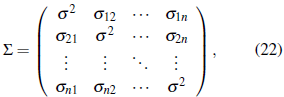
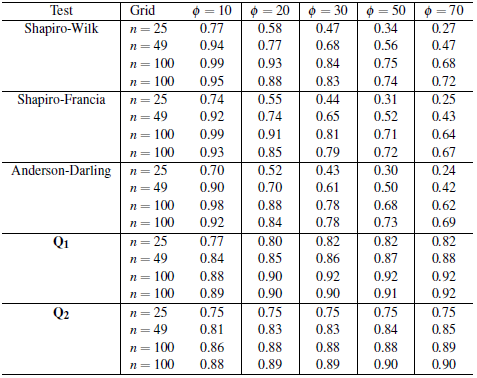
where aij- = C(h) = σ2exp(
 ), σ2, ф > 0, and h = ║xi -xj║, that is, C(Y(xi), Y(x
j)), i, j = 1,...,n, is defined by an exponential model [24]. We consider two values for σ2 (8 and 400) and three values for ф (3, 7 and 12), establishing thus two levels of variability (low and high) and three levels of spatial correlation (low, medium and high), respectively. The models considered are plotted in Figure 2. Combining n (25, 49, 100, 100), σ2 (8 and 400) and ф (3,7, 12) values, in total, we have 24 simulation scenarios. We use the software R [29] to obtain the simulations. The random fields are simulated by using the function grf of the library geoR [30]. The clustered configuration of points is defined by using the function rMatClust of the library sp. The functions shapiro.test, sf.test and ad.test of the library nortest [32] are used to carry out the tests of SW, SF and AD, respectively. The tests based on the Mahalanobis distance (Q1 and Q2) are conducted by using the package base of R [29]. A number of 1000 simulations under each scenario (combinations of n, σ2 and ф) are obtained and the rejection rate for each one of the five tests is estimated by
), σ2, ф > 0, and h = ║xi -xj║, that is, C(Y(xi), Y(x
j)), i, j = 1,...,n, is defined by an exponential model [24]. We consider two values for σ2 (8 and 400) and three values for ф (3, 7 and 12), establishing thus two levels of variability (low and high) and three levels of spatial correlation (low, medium and high), respectively. The models considered are plotted in Figure 2. Combining n (25, 49, 100, 100), σ2 (8 and 400) and ф (3,7, 12) values, in total, we have 24 simulation scenarios. We use the software R [29] to obtain the simulations. The random fields are simulated by using the function grf of the library geoR [30]. The clustered configuration of points is defined by using the function rMatClust of the library sp. The functions shapiro.test, sf.test and ad.test of the library nortest [32] are used to carry out the tests of SW, SF and AD, respectively. The tests based on the Mahalanobis distance (Q1 and Q2) are conducted by using the package base of R [29]. A number of 1000 simulations under each scenario (combinations of n, σ2 and ф) are obtained and the rejection rate for each one of the five tests is estimated by
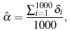
with δi a dichotomous variable taking the value 1 if the null hypothesis is rejected and 0 otherwise. In all cases, the tests are carried out by using a significance level α = 5%, i.e, the test considered is appropriate if the estimation of α (
 ) obtained from the simulation is close to the nominal level 5%. The farther away from this value, the worse its performance. The results of the estimations are shown in Table 1.
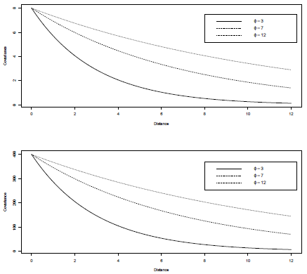
Table 1 Estimated rejection rates (
 ) of the null hypothesis of normality obtained by using Monte Carlo simulation of normal random fields with different levels of variability (σ2) and correlation (ф). In all cases is considered that the process follows an exponential correlation model. The rejection rates are calculated for three regular grids (n = 25,49 and 100) and one clustered grid (n = 100, fourth line at each case).
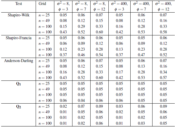
Concerning the univariate tests (SW, SF and AD), several points are identified from Table 1. The estimations of the rejection rates have a very similar behavior (although the values with SF are slightly lower). In general the results are unsatisfactory. It is clear that these tests do not have a good performance because the
 values obtained are greater than the nominal α = 5% defined in the simulations, except in those cases where there is both low spatial dependence (ф = 3) and small sample size (n = 25). It can also be observed that the stronger the spatial dependence, the bigger the difference between σ and a (the higher the spatial correlation, the worse the performance of these tests). A comparison of the α values reported for the three statistics (SW, SF, AD) in the two 100-point spatial configurations (regular and clustered, Table 1) indicates that the magnitude of the error (overestimation of α) increases if a clustered sampling is considered. All the above results are consistent: it is natural that the classical tests are not satisfactory, because they are based on the assumption of independence and the simulations are obtained from normal random fields with an underlying correlation structure.
As for the tests based on the statistics Q1 and Q2, we can observe in Table 1 that in all cases the estimated rejection probabilities (a) (after rounding to two decimal places) are close to the significance level a = 5% considered (particularly when n > 49), i.e. these tests are unbiased [33]. The rejection rates obtained with Q1 indicate that under ideal situations (when the parameters are known), the Mahalanobis distance would perform satisfactorily (as expected in this case all the a values are practically equal to a because the parameters µ and Σ in Equation (17) should not be estimated). Likewise, the rejection rates estimated with Q2, although slightly different from the 5%, are also appropriate (in all cases less than 9%). The relationship between n and a corresponding to the statistics Q2 (for all correlation and variability levels considered) is illustrated in Figure 3. Only the estimations obtained with the regular grids are considered (for the clustered distribution we only have the estimations with n = 100 and these are practically the same as those obtained with the regular grid of the same size). We note according to the interpolations lines in this Figure, that the optimal n is around 50 when ф = 7, while this value is close to 100 when ф = 12, i.e., the greater the spatial dependence, the bigger the sample size required to get a good approximation to the nominal level α = 5% defined in the simulations.
Note from Table 1 that in general (for all the test considered) when n and ф are fixed the estimations of the rejection probabilities obtained under the two levels of variability (σ2 = 8 and 400) are very similar, i.e,
 values in columns 3 and 6, 4 and 7, and 5 and 8 are close. In other words, the variability of the random process has no influence on the result of the normality test. The tests depends only on the number of observations (n) of the random process and the level of spatial correlation (ф). This pattern is apparent in Figure 3 (to the case of Q2), where it can be seen that the variation of
 (with respect to n and ф) is practically the same in both panels (σ2 = 8, above, and σ2 = 400, below).
According to the above comments, the classical tests of normality (SW, SF, AD) should not be used in geostatistics. On the other hand, the test based on the Q1 statistic, although satisfactory, is not applicable in practice because the vector of means and the covariance matrix are unknown. An appropriate test, according to the estimates given in Table 1, is that based on the Q2 statistic. In summary, the estimations based on Q 2 given in Table 1 reveal that this statistic can be used in applied geostatistics for carrying out the normality test and also indicate that its performance depends on the sample size.
4.2 Simulation Under Log-Normality
We also evaluate the power of the test, denoted with n throughout. For this purpose, we simulate data from log-normal stationary processes. Assuming {Y(x),x ∈ ℝ2} is a normal stationary stochastic process with mean µ and variance σ2, a log-normal process can be obtained from Y (x) by means of the transformation T(x) = exp(Y(x)) [24]. It is known that mean and variance of T(x) are given by [26]
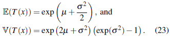
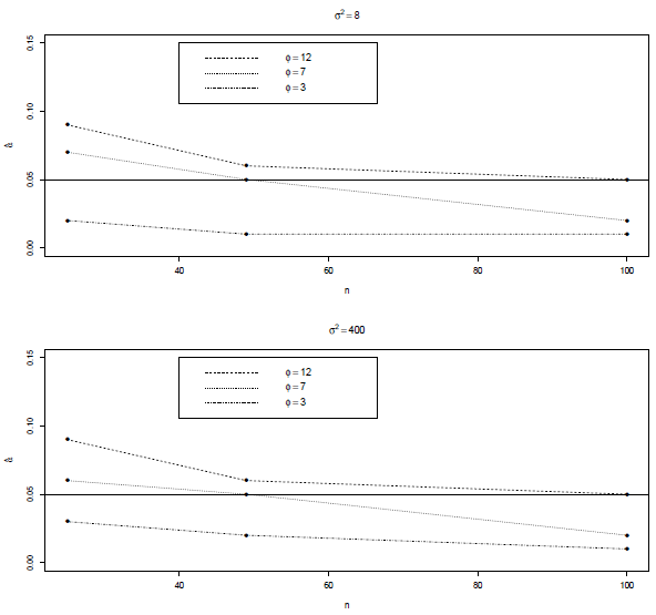
Figure 3 Optimal number of sites (points) required to have a good estimation of a when is used the statistic Q2. Lines calculated only with the estimations of the regular grids.
We use the expressions in (23) to obtain realizations of log-normal random fields starting from simulations of normal processes with µ = 0 and σ = 1. The parameters µ and σ are changed with respect to those used in Section 4.1 for simplicity on the calculations. It is clear that these values have no effect on the estimation of the rejection probabilities
 With these specifications of ß and a we have
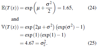
The covariance matrix Σ (see Equation 22) required to calculate the statistic Q1 (Equation 17) for the log-normal processes is based on Equations (24) and (25). The elements of the matrix are now given by
The matrix
 used for obtaining Q
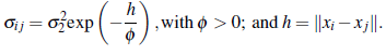
2 is calculated at each case by fitting covariance exponential models by ordinary least squares to the simulated processes (analogously to the procedure used in Section 4.1). Three sample sizes n = (25,49,100) and five correlation coefficients ф = (10,20,30,40,50) are used to evaluate empirically the power of the tests. A size n = 100 clustered configuration (as defined in Section 4.1) is also considered to evaluate the effect of spatial distribution on the estimation of Π. The results are shown in Table 2.
used for obtaining Q
2 is calculated at each case by fitting covariance exponential models by ordinary least squares to the simulated processes (analogously to the procedure used in Section 4.1). Three sample sizes n = (25,49,100) and five correlation coefficients ф = (10,20,30,40,50) are used to evaluate empirically the power of the tests. A size n = 100 clustered configuration (as defined in Section 4.1) is also considered to evaluate the effect of spatial distribution on the estimation of Π. The results are shown in Table 2.
Table 2 Estimated power (
 ) of the normality hypothesis obtained by using Monte Carlo simulation of log-normal random fields with different levels of correlation (ф) and sample size (n). In all cases it is considered that the process has an exponential spatial correlation structure. The power is calculated for three regular grids (n = 25, 49 and 100) and one clustered grid (n = 100, fourth line at each case).
Two points can be highlighted from the
 values. First, the estimations based on the statistics Q1 and Q2 are in general much bigger than derived with the classical tests (except when ф = 10 or both ф = 20 and n = 100) i.e., the tests based on the Mahalanobis distance are more powerful. On the other hand, there are marked differences between trends of change when the level of correlation increases (ф ≥ 30). The three classical tests (SW, SF, AD) show the same pattern. There is an inverse relationship between п and ф, that is, the stronger the spatial dependence, the lower the estimation of the rejection probability (
). On the contrary, in the case of the estimations based on Q1 and Q2 the relationship is monotonous increasing and п is around 90% (when ф = 70 and n = 100 (in both spatial configurations)).
values. First, the estimations based on the statistics Q1 and Q2 are in general much bigger than derived with the classical tests (except when ф = 10 or both ф = 20 and n = 100) i.e., the tests based on the Mahalanobis distance are more powerful. On the other hand, there are marked differences between trends of change when the level of correlation increases (ф ≥ 30). The three classical tests (SW, SF, AD) show the same pattern. There is an inverse relationship between п and ф, that is, the stronger the spatial dependence, the lower the estimation of the rejection probability (
). On the contrary, in the case of the estimations based on Q1 and Q2 the relationship is monotonous increasing and п is around 90% (when ф = 70 and n = 100 (in both spatial configurations)).
Summarizing, the results in Tables 1 and 2 allow us to establish empirically that the classical normality tests such as SW, SF and AD are not appropriate to evaluate this assumption in geostatistics because tend to both overestimate the significance level (a values for these tests in Table 1 are much greater than the nominal level α = 5% considered, particularly when the sample size n and the correlation level ф increase) and underestimate the power (
values in Table 2 for these tests are much lower that obtained with Q1). Results also show that the Mahalanobis distance-based approaches (Q1 and Q2) have a good performance
 values (Table 1) are close to the nominal level α = 5% and the power values п (Table 2) increase as expected when the sample size n and the correlation level ф increase). Consequently the approaches proposed and particularly the statistics Q2 can be applied in practical problems of geostatistics for testing for normality when the process under study is stationary (when simple and ordinary kriging is going to be used to carry out spatial prediction).
Kriging prediction can be applied independently of the distribution that follows the process. However, under normality the prediction is optimal (simple kriging is a BP). In addition to the combination of the method-of-moments and least squares, maximum likelihood can be used to estimate the parameters of the covariance model. This is a straightforward procedure widely used when the random process is normal. For these reasons (optimality and simplicity of estimation) testing for normality is a relevant step in any geostatistical analysis. Classical normality tests based on SW, SF or AD are not suitable in this scenario. The statistics proposed in this work are a good alternative to fulfill this stage of the analysis. Particularly in practical geostatistics, the statistic Q2 can be used in a preliminary step of the analysis for testing for normality.
5 Conclusion and Further Research
In this paper, we introduced an approach to test for normality in geostatistics. Specifically we showed how the Mahalanobis distance, traditionally used in multivariate analysis, can be adapted to a geostatisti-cal context to test for normality. Simulation results indicated firstly that using univariate tests such as Shapiro-Wilk, Shapiro-Francia or Anderson-Darling in geostatistics is inadequate and on the other hand, that the strategy proposed is attractive from a practical point of view because it can be calculated based on just one realization of the underlying random process. There is room for research in the context of this paper. A generalization to the non-stationary case is required. Also the test could be extended to a multivariate geostatistical scenario.

