Services on Demand
Journal
Article
 English (pdf)
 Article in xml format
 Article references
 Send this article by e-mail
Indicators
-
 Cited by SciELO
 -
 Access statistics
Related links
-
 Cited by Google
 -
 Similars in
SciELO
Similars in
SciELO -
 Similars in Google
Share

 Permalink
CT&F - Ciencia, Tecnología y Futuro
Print version ISSN 0122-5383
C.T.F Cienc. Tecnol. Futuro vol.5 no.2 Bucaramanga Jan./June 2013
PRESSURE TRANSIENT ANALYSIS FOR A RESERVOIR WITH A FINITE-CONDUCTIVITY FAULT
ANÁLISIS DE PRESIÓN TRANSITORIA PARA UN YACIMIENTO CON UNA FALLA DE CONDUCTIVIDAD FINITA
Freddy-Humberto Escobar1*, Javier-Andrés Martínez1 and Matilde Montealegre-Madero1
1Universidad Surcolombiana/CENIGAA, Neiva, Huila, Colombia
e-mail: fescobar@usco.edu.co
(Received: Aug. 31, 2012; Accepted: Jun. 06, 2013)
* To whom correspondence should be addressed
ABSTRACT
The signature of the pressure derivative curve for reservoirs with finite-conductivity faults is investigated to understand their behavior and facilitate the interpretation of pressure data. Once a fault is reached by the disturbance, the pressure derivative displays a negative unit-slope indicating that the system is connected to an aquifer, meaning dominance of steady-state flow regime. Afterwards, a half-slope straightline is displayed on the pressure derivative plot when the flow is linear to the fault. Besides, if simultaneously a linear flow occurs inside the fault plane, then a bilinear flow regime takes place which is recognized by a 1/4 slope line on the pressure derivative line. This paper presents the most complete analytical well pressure analysis methodology for finite-conductivity faulted systems using some characteristics features and points found on the pressure and pressure derivative log-log plot. Therefore, such plot is not only used as diagnosis criterion but also as a computational tool. The straight-line conventional analysis is also complemented for characterization of finite- and infinite-conductivity faults. Hence, new equations are introduced to estimate the distance to fault, the fault conductivity and the fault skin factor for such systems. The proposed expressions and methodology were successfully tested with field and synthetic cases.
Keywords: Radial flow, Bilinear flow, Fault conductivity, Steady state.
RESUMEN
Se estudia la huella de la derivada de presión en yacimientos con fallas de conductividad finita para entender su comportamiento y facilitar la interpretación de pruebas de presión. Una vez la perturbación de presión alcanza la falla, la derivada de presión muestra una recta de pendiente de -1 indicando que la falla se conectó a un acuífero y domina el estado estable. Posteriormente, se observa una línea de pendiente ½ en la derivada cuando existe flujo lineal hacia la falla. Si existe flujo simultáneamente dentro del plano de falla, toma lugar el flujo bilineal reconocido por una pendiente de 1/4 en la derivada. El artículo presenta la metodología analítica de pruebas de presión más completa para estos casos, usando características y puntos hallados en el gráfico logarítmico de la derivada. Por ende, el gráfico de la derivada no solo se usa para diagnóstico sino como herramienta de cálculo. La metodología convencional se complementa para caracterizar fracturas conductivas. Se introducen nuevas ecuaciones para determinar la distancia del pozo a la falla, la conductividad de la falla y el factor de daño de la falla para los sistemas en consideración. Las expresiones y metodología propuestas se verificaron satisfactoriamente con ejemplos de campo y sintéticos.
Palabras clave: Flujo radial, Flujo bilineal, Conductividad de falla, Estado estable.
RESUMO
Estuda-se a pegada da derivada de pressão em jazidas com falhas de condutividade finita para entender o seu comportamento e facilitar a interpretação de provas de pressão. Uma vez que a perturbação de pressão atinge a falha, a derivada de pressão mostra uma reta de pendente de -1 indicando que a falha conectou-se a um aquífero e domina o estado estável. Depois, observa-se uma linha de pendente ½ na derivada quando existe fluxo linear para a falha. Se existir fluxo simultaneamente dentro do plano de falha, é o momento do fluxo bilinear reconhecido por uma pendente de 1/4 na derivada. Apresenta-se a metodologia analítica de provas de pressão mais completa para isto, usando características e pontos encontrados no gráfico logarítmico da derivada. Consequentemente, o gráfico da derivada não é usado apenas para diagnóstico, mas também como ferramenta de cálculo. A metodologia convencional é complementada para caracterizar fraturas condutivas. São introduzidas novas equações para determinar a distância do poço à falha, a condutividade da falha e o fator de dano da falha para os sistemas em consideração. As expressões e metodologia propostas foram verificadas satisfatoriamente com exemplos de campo e sintéticos.
Palavras-chave: Fluxo radial, Fluxo bilinear, Condutividade de falha, Estado estável.
1. INTRODUCTION
Many hydrocarbon-bearing formations are faulted and often little information is available about the actual physical characteristics of such faults. Some faults are known to be sealing and some others are non-sealing to the migration of hydrocarbons. While sealing faults block fluid and pressure communication with other regions of the reservoir, infinite-conductivity faults act as pressure support sources and allow fluid transfer across and along the faults planes. Finite-conductivity faults fall between these two limiting cases of sealing and totally non-sealing faults, and are believed to be included in the majority of faulted systems.
A sealing fault is often generated when the throw of the fault plane is such that a permeable stratum on one side of the fault plane is completely juxtaposed against an impermeable stratum on the other side. On the contrary, a non-sealing fault usually has an insufficient throw to cause a complete separation of productive strata on opposite sides of the fault plane. Depending on the permeability of the fault, fluid flow may occur along the fault within the fault plane or just across it laterally from one stratum to another. In general, a finite-conductivity fault exhibits a combined behavior of flow along and across its plane.
While seismic analysis can detect a fault distance to a well with a margin of error near two kilometers, transient pressure analysis is the best tool to detect the distance well-fault with a margin of error of some feet. However, conventionally transient pressure analysis methods have been only used for detection distance fault-well without taking into account such variables as conductivity, damage of the fault and fault length. Before the present work, it was only possible to estimate the fault conductivity using the straight-line conventional analysis with an equation proposed by Trocchio (1990).
Pressure transient analysis offers a possible way to determine the fluid transmissibility of faults. Many models introduced in the literature help characterize faults from pressure transient tests. The simplest of such models uses the well-known method of images for sealing faults. This approach results in doubling the slope of the straight line on a semilog plot of pressure test data. Extensions to intersecting or no intersecting multiple sealing faults have also been reported in the literature. A finite-conductivity fault displays a one-fourth slope on the pressure derivative plot which is equivalent to be identified as a straight line in the Cartesian plot of pressure versus the one-fourth root of time. This behavior was reported by Trocchio (1990) who conducted a study on the Fateh Mishrif reservoir and provided a conventional methodology for determining fracture conductivity and fracture length.
Cinco-Ley, Samaniego and Domínguez (1976) considered the infinite-conductivity fault (or fracture) case and derived an analytical solution for pressure transient behavior using the concept of source functions. They also provided a type-curve matching interpretation methodology. The first attempt to represent a fault as a partial barrier was introduced by Stewart, Gupta and Westaway (1984) who numerically modeled the fault zone as a vertical-semi-permeable barrier of negligible capacity. This model correctly imposed the linear flow pattern at the fault plane. On interference tests, they found that in cases where the conventional method cannot be applied, the inverse problem (non-linear regression analysis) was an excellent approach. Yaxely (1987) derived analytical solutions for partially communicating faults by generalizing the approach presented by Bixel, Larkin, and van Poolen (1963) for reservoirs with a semi-impermeable linear discontinuity. The generated type curves by their solutions yielded separate estimations of the formation transmissibility and the fault transmissibility. Ambastha, McLeroy and Grader (1989) analytically modeled partially communicating faults as a thin skin region in the reservoir according to the concepts of skin presented by van Everdingen (1953) and Hurst (1953). They concluded that for moderate skin values, the pressure response departs from the line-source solution, follows the double-slope behavior for some time, and then reverts back to a semilog linear pressure response parallel to the line-source solution at late time.
The models considered by Stewart et al. (1984), Yaxely (1987), and Ambastha et al. (1989) allow for fluid transfer only laterally across the fault planes. These models do not account for fluid flow along the fault plane which can take place when the permeability of the fault plane is larger than the reservoir permeability surrounding it. A recent model proposed by Boussila, Tiab and Owayed (2003) considers dual porosity behavior in a composite system. All these models neglected the fluid conductance inside the fault along its planes. However, Abbaszadeh and Cinco-Ley (1995) modeled a finite-conductivity fault by specifying the fault parameters with the longitudinal fluid conductance (FCD) and transverse skin factor (sF). These authors neglected the transient nature in the fault zone. They provided some type curves for interference pressure test interpretation.
Anisur-Rahman, Miller and Mattar (2003) presented an analytical solution in the Laplace space to the transient flow problem of a well located near a finite-conductivity fault in a two-zone, composite reservoir. Contrary to previous studies, this solution also considered flow within the fault. They verified their solution by comparing a number of its special cases with those reported in the literature.
The analytical solution reported by Anisur-Rahman et al. (2003) allows us to understand the behavior of a conductive fault. When the pressure disturbance reaches an undamaged conductivity fault, the pressure derivative goes down forming a negative unit-slope line. Since the fault acts as a bridge with an underlying aquifer, steady state flow regime takes place. However, if the fault is damaged and the test runs under radial flow, the pressure derivative rises up more than a log cycle (depending on the damage degree) and once the damaged zone is passed, the pressure derivative goes down, forming the negative unit-slope line. Afterwards, either a half slope or a quarter slope is seen if the conductivity in the fault is either infinite or finite, respectively.
Nowadays, the well test analytical tools are more powerful than many people believe. For instance, conservative well test data interpreters only use the pressure derivative as a diagnosis tool. It means they only use the pressure derivative for distinguishing the several flow regimes for selecting the simulation model to be used, and most of them are unaware that non-linear regression analysis are subjected to none-uniqueness of the solution, which means that there are high possibilities of obtaining inaccurate interpretation results. Precisely, the TDS technique introduced by Tiab (1995) uses characteristic points and lines found on the pressure and pressure derivative curves to estimate reservoir parameters with direct and practical analytical expressions. This technique is used - although without using the appropriate name-in all the most popular commercial software.
This paper uses the solution presented by Anisur- Rahman et al. (2003) to find the characteristic signature observed on the pressure and pressure derivative plot with the purpose of developing appropriate expressions to characterize the typical parameters involved in finite-conductivity faults following the philosophy of TDS technique, Tiab (1995). In this technique, fault damage, fault conductivity and fault length can be easily estimated using data read from the pressure and pressure derivative plot. Furthermore, the well-known straightline conventional methodology was complemented so the above named parameters (fault damage, fault conductivity and fault length) could be easily estimated using the slope and intercept of a cartesian plot. Both provided solutions (TDS and conventional analysis) were successfully verified by its application to actual field and synthetic data.
2. PRESSURE BEHAVIOR OF FINITE-CONDUCTIVITY FAULTS
In the finite-conductivity fault model used by Anisur-Rahman et al. (2003), the fault permeability is larger than the reservoir permeability. Fluid flow is allowed to occur both across and along the fault plane, and the fault enhances the drainage capacity of the reservoir. In their original solution, Abbaszadeh and Cinco-Ley (1995) allowed a change of mobility and storativity in the two reservoir regions. In this study, it is assumed that the reservoir properties are the same in both sides of the fault.
The typical influence of a semi-permeable fault is shown in Figure 1 in which we can observe that the response starts following the usual infinite-acting regime at an early time. Once the finite-conductivity fault is felt by the pressure disturbance, the pressure derivative drops along a straight line of slope -1. The fault provides a pressure support similar to a constant-pressure linear boundary. Later, as the pressure drops in the fault, a flow is established in the thickness of the fault plane which results into a bilinear-flow regime, as depicted in Figure 2. One linear flow takes place in the reservoir when the fluid enters and exits the fault; the second linear flow describes the flux inside the fault thickness. As seen in Figure 1, once the negative unit-slope line disappears as the time progresses, the ¼-slope line develops. Finally, the pressure derivative response becomes again flat describing the infinite-acting radial regime when the fault no longer has effects on the pressure response.
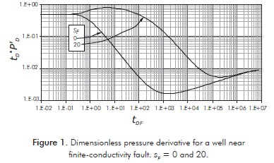
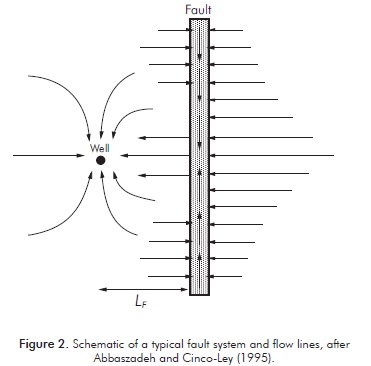
Figure 3 shows the pressure and pressure derivative behavior when the skin factor across the fault plane is equal to zero and the reservoir properties on both sides of the fault are the same. Wellbore storage and wellbore skin effects are not included. Several pressure derivative curves as a function of conductivity of the fault plane, ranging from 0.1 to 107, are shown on this figure. At early times, the pressure derivative is flat representing infinite-acting radial flow in the left-side of the reservoir. At a dimensionless time, tDF, of 0.25, the pressure derivative curves deviate from the radial flow when the pressure transient reaches the fault plane. The deviation degree depends upon the conductivity of the fault plane. For fault conductivities less than 0.1, the pressure derivative essentially remains on radial flow regime indicating that there is no flow along the fault plane and that fluid transfer occurs only across the fault. This is due to the fact that very low fault conductivities create a large flow resistance along the fault plane, while a zero skin factor creates no resistance to flow across the fault. Therefore, fluid flow comes from the right-side to the left-side of the reservoir across the fault, as if the fault plane would not exist.
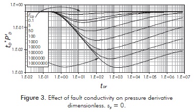
For high-conductivity cases, the fault plane initially acts as a linear constant-pressure boundary and the pressure derivative becomes a straight line with a slope of minus unity. As time progresses, pressure in the fault plane decreases, fluid enters the fault linearly from the reservoir, moves linearly along it, and exits from the fault plane toward the producing well. This flow characteristic is seen as a quarter-slope straight-line bilinear flow regime on the pressure derivative curves. At later times, when the disturbance practically has passed the fault system, the behavior reflects the entire reservoir response and the derivative curves asymptotically reach the radial flow regime again. It is interesting to note that the pressure-transient behavior for intermediate values of fault conductivity is similar to that of naturally fractured reservoirs. Thus, in a pressure test, a single conductive fault can give the appearance of a naturally fractured reservoir.
Figure 4 shows pressure derivative behaviors for finite-conductivity faulty systems under fault skin factor conditions. The reservoir properties are the same everywhere. As expected, the skin creates additional resistance to flow within the fault plane for some period of time, resembling a situation similar to a sealing fault for all conductivity values. Pressure derivatives after the onset of the fault effects tend to approach the well-known behavior of doubling of the semilog straight-line slope (dimensionless pressure derivative equals 1) for sF > 100. At larger times, when pressure on the left side of the fault becomes low enough to allow for appreciable flow to cross the fault plane, the pressure waves propagate through the right-side of the reservoir and the behavior becomes similar to the undamaged fault case, sF = 0. The negative unit-slope line of the constant-pressure linear boundary and the quarter-slope line of the bilinear-flow regime characteristics are developed for high conductivity values, and eventually the dimensionless pressure derivative curves approach the value of 0.5 (combined reservoir behavior).
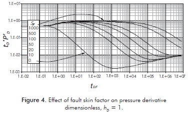
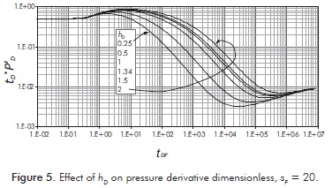
Figure 5 shows dimensionless pressure derivative curves at several dimensionless pay thickness. At low hD, the negative-unit slope line is more visible than at higher values.
3. MATHEMATICAL FORMULATION
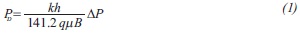
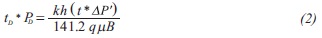
The dimensionless quantities used in this work are defined as:
The formulation of the equations follows the philosophy of the TDS technique, Tiab (1995). It means, several specific regions and "fingerprints" found on the pressure and pressure derivative behavior are dealt with:
1) Permeability and skin factors are found by using the following equations, Tiab (1995):
2) The early radial flow end at:

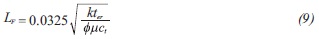
Plugging Equation 3 into the above expression and solving for the distance from the well to the fault:
3) The governing dimensionless pressure derivative for the steady-state flow caused by the fault is:
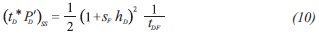
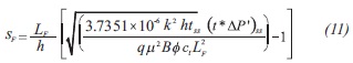
Replacing the dimensionless quantities given by Equations 2, 3 and 4 into Equation 10 and solving for the fault skin factor will result:
4) The pressure and pressure derivative dimension less expressions for the bilinear-flow regime are:
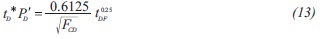
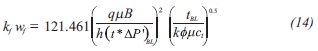
Replacing the dimensionless quantities given by Equations 2, 3 and 5 into Equation 13 will result in an expression to estimate fault conductivity using any arbitrary point on the pressure derivative during the bilinear-flow regime;
5) Using the minimum pressure derivative coordinate, we obtain another expression for the fault conductivity:
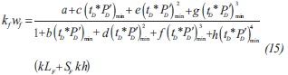
Where the constants are a = 11198700, b = -1235. 2895, c = 256626000, d = 71204.381, e= -491990000, f = 64974400, g = -154650000 and h = 116739000.
6) The dimensionless pressure derivative lines obtained from the radial flow and the steady-state flow Lt regimes intercepts at:

Replacing the dimensionless time into Equation 17 and solving for the well distance to the fault will result in:
7) The line corresponding to the steady state and the bilinear flow line of the dimensionless pressure derivative intersect at:
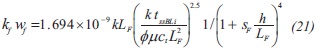
Replacing the dimensionless time defined by Equation 3 into Equation 20 and solving for the conductivity fault will result in:
8) If the dimensionless fault conductivity is bigger than 2.5x10⁸, the bilinear flow disappears and the linear flow appears exhibiting a ½-slope straight line on the pressure derivative curve. In this case we have an infinite-conductivity fault. The dimensionless pressure derivative expression for the above mentioned linear flow regime is:

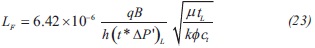
Replacing the dimensionless quantities given by Equations 2 and 3 into Equation 22 will result in another expression useful to estimate the distance from the well to the fault;
New expressions for the straight-line conventional analysis developed in this work are reported in appendix A along with some expressions reported in the literature.
4. EXAMPLES
Example 1
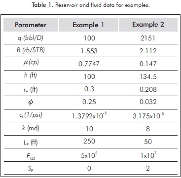
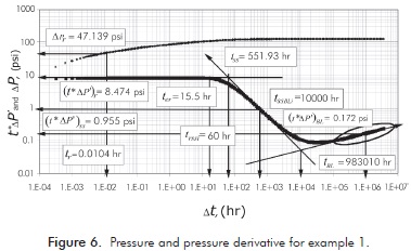
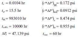
A synthetic pressure test pressure of a well inside an infinite reservoir was generated with the data given in Table 1. Pressure and pressure derivative data are reported in Figure 6. It is required to estimate permeability, skin factor formation, distance to fault and fault conductivity.
Solution
The log-log plot of pressure and pressure derivative against production time is given in Figure 6 from which the following information was read:
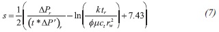
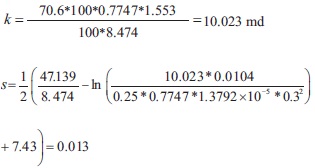
First, the formation permeability is evaluated with Equation 6 and the skin factor with Equation 7:
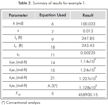
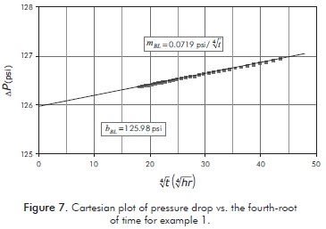
The remaining calculations are reported in Table 2. Furthermore, this example was also solved by the straight-line conventional analysis. For this purpose, only the points falling on the bilinear flow regime (as indicated by the oval in Figure 6) were plotted in Figure 7, from which a slope value of 0.0719 psi/hr0.25 was estimated. Then, Equation A.3 was used to estimate a finite-conductivity value of 1.128x10⁹ md-ft. This value is also reported in Table 2.
Example 2
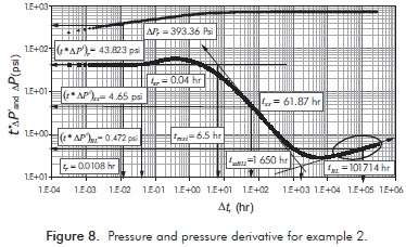
Abbaszadeh and Cinco-Ley (1995) presented well test data from a heavily-faulted carbonate reservoir. Reservoir, fluids and well data are given in Table 1. Pressure and pressure derivative data are reported in Figure 8. It is required to estimate permeability, skin factor formation, distance to fault, fault conductivity and fault skin factor
Solution
The log-log plot of pressure and pressure derivative against production time is given in Figure 7. From that plot the following information was read:
First, the formation permeability is evaluated with Equation 6 and the skin factor with Equation 7 giving value of 7.99 md and - 0.00127, respectively.
A value of 47.54 ft is found with Equation 9 for the distance from the wellbore to the fault. A fault skin factor of 1.91 is estimated with Equation 11. Another value of distance from the wellbore to the fault calculated with Equation 18 results to be 45.92 ft.
The fault conductivity is evaluated with Equation14 and re-estimated with Equations 15 and 21. The respective values are 3.92x10⁹, 3.8x10⁹ and 3.65x10⁹ md-ft. The dimensionless fault conductivity, Equation5, resulted to be 1.032x10⁷.
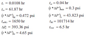
To demonstrate the accuracy of the solution, we also worked this example using conventional analysis and the points indicated by the oval in Figure 9, where the bilinear flow regime takes place. The Cartesian plot of pressure drop versus the fourth-root of time provided a slope of 0.1063 psi/hr0.25, allowing the estimation of a fault's conductivity value of 3.882x10⁹ md-ft which matches very well with the values reported by the TDS technique. This further demonstrates the accuracy of the solution.
5. RESULTS ANALYSIS
For the first example the results agree quite well with the input values for simulation and the fault's conductivity estimated by conventional analysis. The second example provides reasonable results with the work of Abbaszadeh and Cinco-Ley (1995). Also, the conductivity of the fault obtained from conventional analysis matches well with the results of the proposed technique which is considerably enough for accuracy demonstration. Only two examples are reported for space-saving reasons. Although not shown here, the results from conventional analysis, developed in Appendix A, provided reasonable results for fault conductivity, fault skin factor and fracture length.
6. CONCLUSIONS
- Pressure derivative behavior for a well located near finite-conductivity fault was studied and expressions to estimate the distance from the well to the fault, fault conductivity and fault skin factor were introduced and successfully tested with synthetic and field examples. These were also compared to the straight-line conventional technique which complemented this work. It was found that for fault conductivities greater than 2.5x10⁸, the pressure derivative exhibit a half-slope line, since linear flow occurs from the fault to the reservoir. A new expression for this flow regime was introduced, including one to estimate the fault length.
ACKNOWLEDGEMENTS
The authors gratefully thank Universidad Surcolombiana for providing support to the completion of this work.
REFERENCES
Abbaszadeh, M. D. & Cinco-Ley, H. (1995). Pressure-transient behavior in a reservoir with a finite conductivity fault. SPE Formation Evaluation, 10(1), 26-32. [ Links ]
Ambastha, A. K., McLeroy, P. G. & Grader, A. S. (1989). Effects of a partially communicating fault in a composite reservoir on transient pressure testing. SPE Formation Evaluation, 4(2), 210-218. [ Links ]
Anisur-Rahman, N. M., Miller, M. D. & Mattar, L. (2003). Analytical solution to the transient-flow problems for a well located near a finite-conductivity fault in composite reservoirs. SPE Annual Technical Conference and Exhibition, Denver, Colorado, USA. SPE 84295. [ Links ]
Bixel, H. C., Larkin, B. K. & van Poolen, H. K. (1963). Effect of linear discontinuities on pressure buildup and drawdown behavior. J. Pet. Technol., 15(8), 885-895. [ Links ]
Boussila, A. K., Tiab, D. & Owayed, J. (2003). Pressure behavior of well near a leaky boundary in heterogeneous reservoirs. SPE Production and Operations Symposium, Oklahoma City, Oklahoma, USA. SPE 80911. [ Links ]
Cinco-Ley, L. H., Samaniego, F. V. & Domínguez, A. N. (1976). Unsteady state flow behavior for a well near a natural fracture. SPE Annual Technical Conference and Exhibition, New Orleans, USA. SPE 6019. [ Links ]
Hurst, W. (1953). Establishment of the skin effect and its impediment to fluid flow into a wellbore. Pet. Eng. J., 25(11), B6-B16. [ Links ]
Stewart, G., Gupta, A. & Westaway, P. (1984). The interpretation of interference tests in a reservoir with a sealing and partially communicating faults. SPE European Offshore Petroleum Conference, London. SPE 12967. [ Links ]
Tiab, D. (1995). Analysis of pressure and pressure derivative without type-curve matching -skin and wellbore storage. J. Pet. Scie. Eng., 12(3), 171-181. [ Links ]
Trocchio, J. T. (1990). Investigation on fateh mishrif -fluid conductive faults. J. Pet. Technol., 42(8), 1038-1045. [ Links ]
Van Everdingen, A. F. (1953). The skin effect and its influence on the productivity capacity of a well. J. Pet. Technol., 5(6), 171-176. [ Links ]
Yaxely, L. M. (1987). Effect of partially communicating fault on transient pressure behavior. SPE Formation Evaluation, 2(4), 590-598. [ Links ]
APPENDIX A. CONVENTIONAL METHODOLOGY
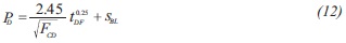
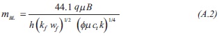
1) Replacing the dimensionless quantities given by Equations 1, 3 and 5 into Equation 12 will result:
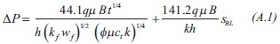
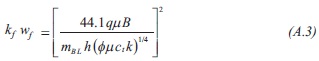
As indicated before, notice that Equation A.1 suggests that a Cartesian plot of ΔPwf vs. t0.25 gives a linear trend which slope allow the estimation of fault conductivity, such as:
The above equation was also found by Trocchio (1990).
2) The dimensionless pressure for the linear flow is:

Replacing the dimensionless quantities given by Equations 1 and 3 into Equation A.4 will result:
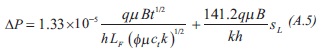
As indicated before, notice that Equation A.5 suggests that a Cartesian plot of ΔPwf vs. t0.5 gives a linear trend which slope allow the estimation for the distance from the well to the fault:
3) The governing dimensionless pressure for the steady state caused by the fault is:
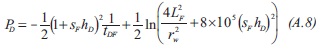
Replacing the dimensionless quantities given by Equations 1 and 3 into Equation A.8 will result:
As indicated before, notice that Equation A.9 suggests that a Cartesian plot of ΔPwf vs. t. 1/t gives a linear trend which slope allow the estimation of fault skin factor.
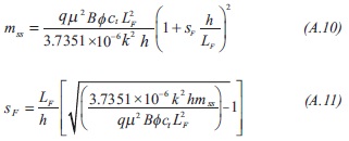
Trocchio (1990) presented the following expression to find the dimensionless end time of the bilinear flow regime and the minimum fracture length:
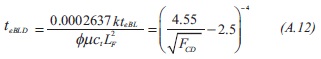
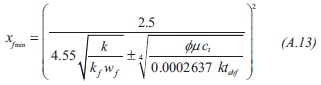
Solving for the minimum fault length: