INTRODUCTION

Marine phytoplankton required nutrients and light for their growth. In the case of light, the signal is absorbed or dispersed by the components present in water, such as colored dissolved organic matter (CDOM); particulates (phytoplankton and detritus), and optically pure seawater. According to ^{Kirk (2011)}, these properties are known as optical properties and are specified in terms of the absorption or dispersion coefficient. They were referred to by ^{Preisendorfer (1961)} as inherent optical properties (IOPs) because their magnitude depends only on the substances present in the aquatic environment and not on the geometric structure of the light fields that can penetrate the water column (^{Mobley, 1994}; Kirk, 2011). The science that is in charge of studying them is hydrological optics, which is a part of physics that studies the behavior of light in water (Kirk, 1994).

IOPs have been used in the validation of ocean color satellite products (IOCCG, 2006; ^{Brewin et al., 2015}). These components absorb light at different wavelengths of the electromagnetic spectrum (^{Sathyendranath and Morel, 1983}), allowing differentiation of absorption spectra that in the case of water, it registers greater absorption in red, for CDOM in ultraviolet-visible and particulate material such as phytoplankton in the blue (^{Aguilar-Maldonado et al., 2018}a).

Changes in ocean color can be measured through traditional techniques (in situ sampling) (Santamaría-del-Ángel et al., 2015; ^{Aguilar-Maldonado et al., 2018}a) or satellite platforms (Aguilar Maldonado et al., 2018b; Aguilar-Maldonado et al., 2019). In the case of traditional samplings, there are few optical properties database programs (Santamaría-del-Ángel et al., 2015), while methods with ocean color satellite platforms have been concerned with incorporating new products to understand the characteristics of absorption, dispersion of water and its constituents (Aguilar-Maldonado et al., 2019), although in the beginning the missions were oriented only to the determination of the concentration of Chlorophyll-a (Ch-a) in the oceans (^{Arnone et al., 2006}; IOCCG, 2015).

Within the documented events, which change the color of the ocean, are the phytoplankton blooms, which respond to natural or seasonal events and play an important role in local ecological balances (^{Falkowski and Raven, 2007}). When a bloom occurs, depending on the dominant group that generates it, the color can change from a bright green to red or dark brown (Santamaría-del-Ángel et al., 2015). The color of the bloom is the result of the pigments contained within the phytoplankton cells, together with other factors such as sediments, CDOM, and any other compound present in the water plot (Barocio-León et al., 2006).

Phytoplankton blooms can be characterized with methods other than the traditional ones, Santamaría-del-Ángel et al. (2015) proposed the use of a IOP_Index to detect blooms in optically complex waters. This IOP_Index is calculated from the spatial standardized anomalies of the absorption coefficients of phytoplankton (a_phy), of the colored dissolved organic matter (a_CDOM), and the detritus (a_d, non-algal particles), using the wavelength (λ) 443 nm. It also considers the analysis of orthogonal empirical functions, following the criteria outlined by Santamaría-del-Ángel et al. (2011) and can classify the stations under conditions of bloom or non-bloom.

In Antarctica, blooms develop from spring to summer. Research carried out in the ‘70s (^{Holm-Hansen et al., 1989}), showed that most of the Antarctic oceanic water masses predominated with low phytoplankton biomasses, where the fraction of micro-phytoplankton was much lower than that of nanophytoplankton, but in the coastal areas this biomass increased. Changes in the composition of phytoplankton in the West Antarctic Peninsula (WAP), from large diatoms (^{Rodriguez et al., 2002}) to small cryptophytes (^{Mendes et al., 2018}) have generated consequences in the upper trophic levels (Mendes et al., 2013). To date, with IOPs, bloom conditions have not been documented for this area, but have been carried out through satellite platforms using the concentration of chlorophyll-a (Chl-a) as an indicator (^{Gonçalves-Araujo et al., 2015}) and in situ databases, with which five-year cycles (^{Saba et al., 2014}; ^{Kim et al., 2018}) were detected in the increases in phytoplankton biomass.

Therefore, the objective of this work was to characterize blooms of phytoplankton in the EG using the IOP_Index proposed by Santamaría-del-Ángel et al. (2015). For this, surface stations were considered and in the MPC in 2017 and 2018, each year and depth was considered separately. Also, the IOP_Index was related to the size structure (picophytoplakton, nanophytoplankton or microphytoplankton), to identify the size fraction of the phytoplankton responsible for the blooms, an aspect not addressed to date in this geographical area of study.

STUDY AREA

The EG is located in the coastal zone of the Western Antarctic Peninsula and north of the Palmer Archipelago (^{García et al., 2002}; Varela et al., 2002), it is a shallow basin limited to the west by the Anvers and Brabant islands and the East with the North Antarctic Peninsula. It is connected to the north with the Bransfield Strait and the Bellingshausen Sea through two narrow channels, in the center by the Schollaert Canal and the south by the Bismarck Canal (^{Kerr et al., 2018}). They are considered to be a westward extension of the Western Basin of the Bransfield Strait (García et al., 2002; ^{Rodriguez et al. 2002}) (Fig. 1).

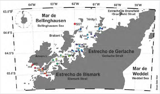
Figure 1 Distribution of stations in the Strait of Gerlache. The southern region was represented by the stations of red circles (2017) and orange (2018), the central region dark green circles (2017) light green (2018), and the northern region blue circles (2017) and purple (2018). 

Circulation studies (^{Doval et. Al., 2002}; ^{Zhou et al., 2002}; Sagra et al., 2011) in the EG indicate the incidence of water bodies from the Weddell, Bellingshausen, and Drake Seas. The predominant water bodies are transitional zonal waters influenced by the Bellingshausen Sea (TBW) that flow through different pathways such as the Bismark and Dalman Straits through the Shorlaert Channel Bay and transitional zonal waters influenced by the Weddell Sea (TWW) (^{García et al., 2002}). Surface circulation varies by season, with a main northward outflow pattern (Zou et al., 2002) joining the flow of the Bransfield Current, a western boundary current moving northeast near the South Shetland Islands (Sagra et al., 2011).

MATERIALS AND METHODS

Samples of water on the surface and the maximum of Chl-a (MPC), depth at which the highest concentration of Chl-a occurs, were collected through an oceanographic rosette system of 12 bottles of 8 L each. Fluorescence profiles were taken at the stations to identify the MPC with an ECOtriplet fluorimeter coupled to a CDT SB 19 Plus. These samples were taken during the third (January 2017) and fourth expedition (January 2018) from Colombia to Antarctica (Fig. 1) in the EG, within the framework of the Project: Marine scientific research for maritime safety in Antarctica” By the General Maritime Directorate.

Between 1 to 2 L of water were filtered through GF / F filters, with a positive filtration system, to determine the absorption coefficients by the particulate material (a _P(λ)), according to ^{Mitchell et al. (2002)}. Filters were stored in histoprep capsules and liquid nitrogen until laboratory analysis. Additionally, samples of 250 mL of water were taken, in amber bottles previously treated with 10 % HCL and muffled at 450 °C, to determine a _CDOM (λ) according to Mitchell et al. (2002).

In the laboratory, for the determination of a _P(λ), the filters were moistened with a drop of filtered seawater, and their optical density (OD) was read between 400 to 700 nm with 1 nm increments, through a Varian spectrophotometer. -Cary 100 with an integrating sphere system following the protocol of ^{Mitchell et al. (2002)}. The reading procedure was repeated after rinsing the filters twice, with hot methanol for 15 minutes, to obtain the detritus absorption coefficient a _d(λ). The phytoplankton absorption coefficient a _Phy(λ) was obtained by the difference between a _P (λ) and a _d (λ).

For the determination of a _CDOM (λ), the water samples were filtered through membrane filters of 0.25 mm pore and the optical density of the filtrate was read between 250 to 750 nm, using cells of 10 cm in length. The determination a _CDOM (λ) was made according to ^{Mitchell et al. (2002)}.

To identify the state of the stations bloom sampled in the EG, the IOP_Index was calculated for stations on the surface-2017, in the MPC-2017, on the surface-2018, and in the MCP-2018 according to Santamaría-del-Ángel et al., (2015), whose process involved: 1) standardizing the values of a _Phy (443), a _CDOM (443) and a _d (443), through the Z transformation; 2) perform principal component analysis to reduce the number of variables; 3) choose the first ACP because it represents the greatest possible variation of the data set based on the proper values (eigenvalues and 4) calculate the index based on the first standardized orthogonal empirical function (SEOF1) (Santamaría-del-Ángel et al., 2011) by:

Where Z corresponds to the standardized spatial anomalies by condition (surface 2017, MPC 2017, surface 2018, and MPC 2018) of the absorptions of a _Phy (443), a _CDOM (443), and a _d (443) respectively and the coefficients b _1,1 , b _1,2 , and b _1,3 to the weights of the anomalies. To describe the state of bloom, the criterion of Santamaría-del-Ángel et al. (2015), who indicated that in a Gaussin distribution, a 95 % confidence interval has an upper limit of 1.96 standard deviations ( Z value). This value was rounded to 2 standard deviations to define the limit of conditions of bloom. The higher this value the more intense the bloom will be. Based on the above, ^{Aguilar-Maldonado et al. (2018}b), to describe the stages of a phytoplankton bloom, they interpreted the IOP_Index values defining values, <than 1, the season is in non-bloom conditions; Values between 1 and 2 represent conditions in which the station is about to enter conditions bloom or is already emerging from bloom, and values higher than 2 are anomalous and indicate active bloom conditions.

On the other hand, with the a _Phy (λ), it is also possible to determine the size index of the dominant phytoplankton population (^{Wu et al., 2007}; ^{Millan-Nuñez and Millan-Nuñez, 2010}) in cruise ships, using the ratio:

With the Blue / Red ratio it was possible to identify the size fraction of the phytoplankton population responsible for bloom by relating it to the IOP_Index. According to, ^{Wu et al. (2007)}, a ratio of Blue / Red greater than 3.0 implies the predominance of picophytoplankton and values of less than 2.5 of microphytoplankton, so that the interval between 2.5 and 3.0 would predominate nanophytoplankton (Santamaría-del-Ángel et al., 2015).

RESULTS AND DISCUSSION

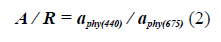
The advantage of using this index is that it does not depend on the number of observations; therefore, it is a good method to compare research campaigns that have different numbers of samples (Santamaría-del-Ángel et al., 2015). For 2017, the IOP_Index (Figs. 2a, 2b) showed four stations in bloom conditions, three in conditions of entry or exit of bloom, and twelve in non-bloom conditions. Previous studies (^{Holm-Hansen et al., 1989}; ^{Figueroa, 2002}; ^{Rodriguez et al., 2002}), indicated that it is a highly productive area, with a wide spatio-temporal variation in phytoplankton production, due to increased stability in the surface layer as a consequence of the glacial contribution. The above, coupled with mixing processes reduced by the protected geomorphology of this area, leads to the generation of phytoplankton blooms (Varela et al., 2002) that sustain all the higher trophic levels. Likewise, this high productivity is attributed, among other factors, to the complex pattern of circulation, the dynamics of ice, the entry of continental water, and the different bodies of water that converge in it (^{Kerr et al., 2018}).

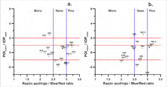
Figure 2 Relationship of the IOPIndex with the size structure to identify blooms in Stations: a. superficial 2017, b. in the MPC in 2017. 

The stations identified in bloom conditions, on the surface of 2017, were D04 located at Palmer Station south of the EG and G16 station also located in the South of the Strait (Fig. 2a). For this condition, the scatter diagram of the IOP_Index vs the Blue / Red ratio showed that the size structure that made up the bloom in these two stations was the micro-plankton (Fig. 2a). The works of ^{Rodriguez et al. (2002)} and Varela et al. (2002), for coastal areas of the EG, described that a wide spatio-temporal variation of phytoplankton production occurs together with high concentrations of Chl-a and dominance of diatoms (^{Mendes et al., 2013}; ^{Gonçalves-Araujo et al., 2015};), which continues to maintain micro-plankton size structures according to the IOP_Index approximation.

It was possible to compare the magnitude of the absorption spectrum of the bloom Stations through the calculation of the dimensionless spectrum (A) according to the criteria of Barocio-Leon et al. (2006). With the A spectrum, the differences in the magnitude of the spectra generated by the chlorophyll concentration of each sample are eliminated. Therefore, each absorption value between 400 to 700 nm was standardized by the maximum absorption value of this interval. In the case of the D04 station, a pronounced shoulder was not observed between 480 to 500 nm (Fig. 3b), these differences in shape are attributed to variations in the concentration and composition of pigments present in the cell (^{Babin et al., 2003}) or the packet effect, due to cell size (^{Wright and Jeffrey, 2006}).

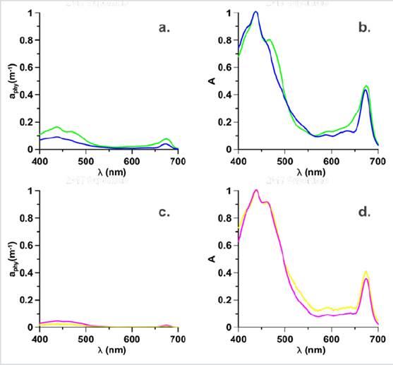
Figure 3 Absorption coefficients of Phytoplankton and Normalized absorption spectra (adimensional), where the 2017 surface Stations: G16 (green), D04 (Blue) in bloom are represented in a. aphy spectrum, b. Normalized spectrum and for the bloom stations in the MPC in 2017: G04 (yellow), H01-3 (magenta) are represented in c. aphy spectrum and d. Normalized spectrum. 

High-performance liquid chromatography data (HPLC, ^{Thomas et al., 2012}) showed that at G16 station, the highest concentration of pigments was fucoxanthin, which is the marker pigment of diatoms (^{Roy et al., 2011} ), while, at station D04, similar concentrations of fucoxanthin, hexfucoxanthin and, to a lesser extent, alloxanthin were observed (Fig. 4). The foregoing shows a change in the concentration of pigments and therefore, in the composition of the phytoplankton structure (^{Sathyendranath et al., 2001}; Cañon-Páez, 2020) in these two seasons in active bloom. Likewise, in the region between 550 and 650 nm (Fig. 3b), the absorption is lower, and with shoulders not observed in the G16 station, these forms are characteristic of groups with the presence of carotenoid pigments (^{Wright et al., 1991}).

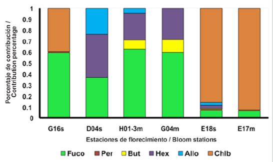
Figure 4 Percentage of the pigments fucoxanthin (Fuco), peridinin (Per), butanoyloxyfucoxanthin (But), hexanoyloxyfucoxanthin (Hex), alloxanthin (Allo), chlorophyll b (Chl-b) contribution, in the bloom stations where: 2017 on the surface (G16, D04) and MPC (H01-3, G04); 2018 on the surface (E18) and in MPC (E17). 

In contrast, the 2017 surface station G08, located in the northern region of the Strait, was identified in a bloom condition for picophytoplankton (Fig. 2a), but apparently in an exit bloom condition. This result reveals an advantage of the method, in that, with the IOP_Index it is possible to identify whether or not a station is in bloom conditions, it also allows us to identify blooms caused by the different sizes of phytoplankton, which is not possible to observe with traditional methods such as microscope observation.

In the MPC stations in 2017, the IOP_Index showed station G04, in a bloom state caused by microphytoplakton (Fig. 2b), while in station H01-3 it was also in bloom but of nanophytoplankton (Fig. 2b). An important aspect to highlight, given that the report of blooms for fractions such as nano or picophytoplankton is scarce, due to the limitations of the traditional method of observing small fractions (Santamaría-del-Ángel et al., 2015). For the stations identified in conditions of entry or exit of bloom, which were two, in sampling point H01-2 the responsible fraction was picophytoplankton, and in H02 nanophytoplankton, the others were presented in non-bloom conditions (Fig. 2b). However, low CDOM values for stations H01-2 and H02 (0.02 and 0.03 m^-1) indicate that the condition for these stations is at the beginning of bloom.

One aspect to observe is that stations G04 and H01-3 were identified on the surface as non-bloom stations, which constitutes another advantage of this method since it allows the identification of conditions of bloom in-depth or subsurface bloom. Furthermore, this result suggests that during 2017 the surface was not interconnected with the MPC, each one acting independently. This suggests a high glacier contribution with greater stratification in the water column, as a result of the increase in meltwater in a warm year (^{Kim et al., 2018}), which causes the stability in the surface layer to increase as a consequence of the glacial contribution and coupled with reduced mixing processes (Varela et al., 2002), leads to the generation of independent phytoplankton blooms.

If the magnitude of the a_phy spectra is observed, of the stations G04 and H01-3 in the MCP in 2017 (Fig. 3c) they are more flattened, with respect to the spectra of the bloom stations (G16, D04) on the surface in 2017 (Fig. 3a). The explanation for this flattening may be due to the adaptation of phytoplankton communities to photoacclimation processes, or due to the pigment packaging effect, which is the characteristic of communities with larger cell sizes (^{Bricaud et al., 1995}) and that generally they are evidenced by the flattening of the absorption spectrum. Both photoacclimation and the packaging effect cause the phytoplankton communities to regulate the pigment content in the cell in response to the availability of light (^{MacIntyre et al., 2002}) causing a change in the shape (Fig. 3d) of the spectrum (Bricaud et al., 2004).

In addition to the above, in Figure 4, it is observed that the concentration of pigments differs in the stations of the surface and the MPC, an aspect that also influences the change in the shape of the spectra (Fig. 3d). Therefore, unlike the surface in the MPC, the bloom stations presented structures of different sizes and composition of pigments that show changes in the phytoplankton structure causing the bloom (Cañon-Páez, 2020).

The normalized spectra presented in stations G04 and H01-3 (Fig. 3d) did not present differences in the shoulder between 480 and 500 nm, being very similar, however, the magnitude of absorption between 500 and 650 nm was lower for the station H01-3. This change may be the product of the presence of Allo, a pigment associated with Hex with nanophytoplankton (^{Vidussi et al., 2001}). Therefore, it is suggested that in the MPC, the change in the shape of the spectra was due to the cell size that influences the packaging effect (^{Bricaud et al., 2004}), to photoacclimation processes (^{Ciotti et al., 2002}; Barocio-León et al., 2006;) and the differences in the proportions of phytoplankton pigments present in the communities present in the bloom stations.

As for the 2018 data, only two stations (E18, E17) were identified in bloom conditions, two in conditions of entry or exit of bloom (E05, E06), and nine in non-bloom conditions (E13, E04, E01, E03, E10, E28, E22, E08, E09) (Figs. 5a and 5b). Of the stations identified in surface bloom, only E18 was observed in micro-plankton bloom (Fig. 5a). Stations E17, E05, and E06 were identified in conditions of entry or exit of bloom, also with a predominance of micro-plankton.

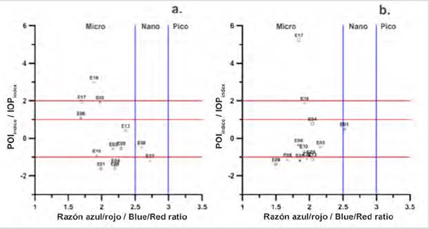
Figure 5 Relation of the IOPIndex with the size structure to identify blooms in Stations: a. superficial 2018, b. in the MPC in 2018. 

Stations E17 and E05 on the surface in 2018 were close to the lower limit to be considered in bloom conditions, with a value of 1.9 (Fig. 5a), so it would be thought that this station is in the process of starting a bloom or just coming out of it. To identify whether the bloom is beginning or is in decline, it would be expected to find high values of a_CDOM (443) if it were the second option, since according to ^{Aguilar-Maldonado et al. (2018}a) a source of CDOM in a bloom, is constituted by phytoplankton in decomposition processes, associated with the most intense stage of the previous bloom. It has also been reported that other sources of CDOM in Antarctic waters are bacterioplankton and Krill (^{Ortega-Retuerta et al., 2010}; 2009). In the case of stations E17 and E05, they presented CDOM values of 0.12 m^-1 (which represents a standardized anomaly Z = (-0.87) and of 0.25 m^-1 (Z = 1.14), respectively. These values suggest that season E05 is in the decline phase of bloom, while season E17 is just beginning.

Station E18 showed the a_phy (λ), below 0.2 m^-1 (Fig. 6a) and its normalized spectra (Fig. 6b) revealed a pronounced shoulder in the region 480 at 500 nm which was not observed in the bloom station in 2017. This shoulder is the characteristic of populations with the presence of Allo and Hex (^{Cota et al. 2003}), which generates changes in the absorption spectrum of this season to those of 2017. In Figure 4 high contributions of Chl-b can be observed for this sampling point, a pigment not observed in the bloom stations in 2017 and which is considered a marker of chlorophytes (^{Roy et al., 2011}). Due to the high concentration of this pigment, it would be thought according to Vidusii et al. (2001) that the size fraction responsible for bloom would be nanophytoplankton, however, the Blue / Red Ratio proposed by ^{Wu et al. (2007)}, let us see with the index that corresponds to micro-plankton. With this station, it was also possible to observe the change in the structure of the phytoplankton community in the EG between 2017 and 2018, observed in the form of the spectra (Figs. 3 and 5), which may be associated with different physiological responses of the communities by environmental factors (^{Gonçalves-Araujo et al., 2015}) and ecological factors, including different degrees of pigment packing (Ferreira et al., 2018).

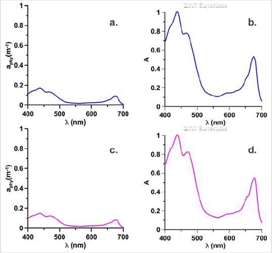
Figure 6 Absorption coefficients of Phytoplankton and Normalized absorption spectra (adimensional), for the bloom stations in 2018: Surface of the E18 (Blue) are represented in a. aph spectra, b. Normalized spectra and for the E17 (magenta) MPC it is they represent in c. aph spectra and d. Normalized spectra. 

On the other hand, in the MPC stations in 2018, station E17 reached an IOP_Index value of 5 (standard deviations), showing this station in a very intense bloom state, caused by micro-plankton (Fig. 5b). This confirms that this station on the surface was not at the end of the bloom but at the entrance, due to the value of the IOP_Index registered for the MCP and the low values of CDOM. On the contrary, the station E18, by the value of the IOP_Index for the MPC, would indicate the exit condition of the bloom due to the increase in the value of the CDOM (0.22 m^-1) with respect to the surface (0.18 m^-1).

With stations E17 and E18, an interconnection between the surface and the MCP is evidenced in 2018, unidentified in 2017, where the bloom stations in the MPC were different from those on the surface, suggesting less glacial contribution, thus stratification in the water column was smaller and the interconnection was more evident. Therefore, greater mixing processes are suggested in 2018 that involve interconnected layers between the surface and the MPC that are not independent as in 2017. Also, station E17 presented the absorption spectra with the highest absorption magnitudes, noting a pronounced shoulder between 450 and 500 nm (Fig. 6c) and in the adimensional spectra the shape is very similar to the E18 on the surface, however, the shoulder is more pronounced in the E17. The difference is due to the presence of other pigments in E18 (Fig. 4) such as Allo and Hex. In E17, Chl-b was the pigment with the highest concentration, for which it would be thought that the group with the greatest contribution to bloom in this sampling point would be given by the green flagellates (chlorophytes) and not by diatoms (^{Mendes et al., 2012}) that were present in 2017 due to the contribution of fucoxanthin as shown in Figure 4.

The differences observed in the community structures, responsible for the blooms in 2018 compared to 2017, maybe due to the environmental variability already identified by ^{Kim et al. (2018)} for the POA, where cycles of high chlorophyll concentration are observed every 5 years, with 2017 being a year with high biomass (1.22 mg/m³ Chl-a and 1.42 mg/m³ Chl-a, on the surface and in the MPC) and 2018 would be identified as the beginning of the period in biomass decline (0.63 and 0.70 mg/m³ Chl-a on the surface and the MPC).

CONCLUSIONS

In this work, through the IOP_Index, it was possible to identify surface and subsurface blooms (in stations H01-3, G04, and E17 of the MPC) in the EG, observing changes in the conditions studied, where in 2017 it was not possible to observe an interconnection between the surface stations and the MPC, while in 2018 it did. Changes in the shape of the absorption spectra showed variations in the phytoplankton structure due to size structure, the composition of different pigments, and warm (2017) and cold (2108) environmental conditions. This approach allowed the identification of peak and nanophytoplankton blooms that cannot be observed using the traditional method since these size structures are not identifiable in the traditional light microscope. This makes this tool a very important complement in monitoring programs where the phytoplankton component is considered.