


Services on Demand
Journal
Article
 English (pdf)
 Article in xml format
 Article references
 Send this article by e-mail
Indicators
-
 Cited by SciELO
 -
 Access statistics
Related links
-
 Cited by Google
 -
 Similars in
SciELO
Similars in
SciELO -
 Similars in Google
Share

 Permalink
Ingeniería y competitividad
Print version ISSN 0123-3033
Ing. compet. vol.17 no.2 Cali July/Dec. 2015
Measuring financial risk in non-financial firms: an application to the Colombian sugar sector
Medición de riesgo financiero en empresas no financieras: una aplicación al sector azucarero colombiano
Stephanía Mosquera-López
School of Industrial Engineering, Faculty of Engineering, Universidad del Valle. Cali, Colombia
E-mail: stephania.mosquera.lopez@correounivalle.edu.co
Eje temático: INDUSTRIAL ENGINEERING / INGENIERíA INDUSTRIAL
Recibido: Enero 14 de 2015
Aceptado: Julio 1 de 2015
Abstract
Investment projects optimal selection is relevant in making business decisions. In this paper a methodology that has not been extensively explored in the literature of measuring financial risk is applied to the Colombian sugar industry. This measurement serves as the basis for the evaluation of projects in a more robust manner, due to an adequate modeling of uncertainty. For the above, the Value at Risk of a company's gross profit is determined using econometric techniques such as modeling the autoregressive conditional volatility of the series, multivariate modeling of the dependency relationships of the series through copulas, and simulation using Monte Carlo techniques.
Keywords: Copulas, EVT, sugar market, VaR.
Resumen
La selección óptima de proyectos de inversión es de gran importancia en la toma decisiones de las empresas. En el presente documento se realiza una aplicación en el sector azucarero colombiano de una metodología que aún no ha sido ampliamente explorada en la literatura de medición del riesgo financiero. Esta medición sirve como base para realizar valoraciones de proyectos de una manera más robusta, al modelar adecuadamente la incertidumbre. Para lo anterior se calcula el Valor en Riesgo de la utilidad bruta de una empresa del sector, indicador que se estima haciendo uso de técnicas econométricas como la modelación de la de volatilidad condicional autoregresiva de las series, así como la modelación multivariada a través de cópulas de las relaciones de dependencia entre éstas y, de la simulación de escenarios mediante técnicas de Monte Carlo.
Palabras Clave: Cópulas, mercado del azúcar, TVE, VeR.
1. Introduction
The optimal selection of investment projects within companies is part of their tasks and goals, hence their profitability depends of an appropriate choice. For this reason the study of optimal selection of investment alternatives is a subject of interest for practitioners and academic research. Traditionally, from economic engineering and corporate finance analysis, different models and indicators have been used to determine the feasibility of investment projects in enterprises. The most commonly used indicators are the Net Present Value (NPV), internal rate of return (IRR), modified internal rate of return, the expected value of future cash flows, among others.
However, this approach to project management within companies is completely deterministic, because it does not consider the stochastic nature of some variables (risk factors) that affect the profitability of the projects. Thus, this paper aims to apply a new methodology for measuring financial risk, which permits taking investment decisions based on more robust valuations.
The methodology used in this study takes into account the non-deterministic nature of variables, both internal and external to the company, that affect its profitability. Variables such as international commodity prices, market reference rates or exchange rates. For this, econometric techniques that have not been widely used in the literature are applied. The techniques allow an adequate modeling of the key variables within the financial and operational structures of companies.
In Manotas (2009) and Manotas & Toro (2009) the authors present proposals for the analysis and modeling of uncertainty in the context of project portfolio selection. The first makes an analysis of economic selection of projects under uncertainty, and in the second the authors propose the concept of NPV at risk, as a natural extension of VaR (value at risk), with applications to the sugar sector.
Nevertheless, the application of advanced econometric techniques to build robust feasibility indicators by modeling uncertainty for project valuation is still incipient in the literature. In Uribe, et al., (2015), the authors propose a methodology to construct a feasibility indicator of this type. This indicator is the VaR constructed using econometric techniques such as modelling the autoregressive conditional volatility of the series, the multivariate modeling of the dependency relationships between them through copulas, and scenarios simulation using Monte Carlo techniques. The authors apply empirically their methodology in a Colombian exporter company of the gold sector.
>Regarding to the application of advanced econometric techniques and financial engineering for the modeling of risk (but not in the context of optimal selection of investment projects) there has been a high productivity in recent literature. Most papers model the risk by building a VaR with application in electricity prices, carbon emission permits or derivatives prices.
Xiong & Zou (2014) perform a literature review of methodologies to model the volatility of electricity prices. In general, there are four approaches in the literature for modeling the volatility of different prices' series, these are: the parametric approach, nonparametric approach, semi-parametric approach and computational approach.
The parametric approach requires assumptions about the statistical distribution that the data follow. The methodologies used in this approach are GARCH (Generalized autoregressive conditional heteroskedasticity) and calculating the VaR with EWMA (Exponential Weighted Moving Average) method proposed by RiskMetrics. Chevallier (2011), Feng, et al., (2011), Zhang, et al., (2013) and Hai & Yang (2014) model the volatility in carbon prices using this approach. As for electricity prices, Cifter (2013) also models them following a parametric approach.
The nonparametric approach is based on historical data or simulations to measure risk, therefore it is easy to implement. Within this approach historical simulation techniques and Monte Carlosimulation are found. This approach is used in Manotas (2009) to risk measurement in a company of public services. The semiparametric approach does not require strict assumptions about the distribution of the data, but keeps the advantages of the most used parametric methods. The works of Feng, et al., (2012), Wang & Wang (2014), Yang & Lin (2011) are within this approach. The authors make use of GARCH, EVT (Extreme Value Theory) and copulas to model the volatility of carbon prices, electricity prices and rubber futures.
The computational approach is based on Fourier analysis techniques, wavelet analysis, and empirical mode decomposition. Yang & Lin (2011) and Wang, et al., (2014) also apply some of these techniques.
The methodology used in this research lays in the semiparametric approach. It is considered an appropriate approach because the risk factors are on a daily basis. The stylized facts of financial series are taken into account by the use of ARIMA-DCC-GARCH models and extreme value theory, facts as volatility clusters and heavy tails. Yet, the effect of the risk factors effect must not be quantified separately, since they are correlated (linearly and non-linearly). Thus, the co-movement of the factors is what must be considered. The use of copulas enables us to model the multivariate distribution of risk factors, in order to obtain their dependence relationships.
Therefore, the contribution of this study is the application of advanced econometric techniques, that despite they have been explored in other application areas, have not been used in measuring financial risk for feasibility evaluation of investment projects, evaluations that are made with more robust indicators like the VaR of output variables.
This methodology is applied to a company in the Colombian sugar industry, a sector of great importance for the economy of the country and the region. The sector had a production in 2013 of 2.13 million tons of sugar, recording an annual increase of 2.4% compared to 2012. In addition, the sugar industry generated more than 180,000 jobs in the first links of its production chain.
Internationally, global sugar production in 2013 was of 173 million tons. Colombia's participation in the production was only of 1.14%, hence Colombia is a price taker in this market. Additionally, most of the international transactions of sugar futures are made in the stock exchanges of New York and London, negotiations that determine the international sugar price.
This document is structured as follows: Section 2 describes the methodology used; Section 3 presents the results obtained; Section 4 concludes the study; Section 5 presents the bibliographical references.
2. Methodology
Following Manotas (2009), the construction of a company's risk assessment model begins with the definition of the input variables, which condition the feasible model results. The input variables can be external (macroeconomic, related to the market, industrial sectors, etc.) or internal (inventory policies, levels of efficiency, production issues, etc.).
In addition, an output variable which is endogenous to the enterprise (such as income, expenses, EBITDA, etc.) must be determined. This variable is chosen according to its exposure to the risk factors, that is the input variables.
Subsequently it is necessary to establish the relationships between the variables, thereby making it possible to define the future cash flows of the project. Once the cash flow is calculated decision criteria such as NPV, IRR, the modified IRR, among others, can be implemented.
In the present study we will take into account external factors, specifically macroeconomic and financial. For example, the exchange rate, commodity spot and futures prices. To determine the relationship between the risk factors the methodology outlined by McNeil, Frey & Embrechts (2005) is followed, obtaining the relationship between them by using copulas and EVT.
The use of copulas, EVT and traditional techniques in time series econometrics, such as Autoregressive integrated moving average models (ARIMA), for the forecast of risk factors in the context of valuation of projects is proposed by Uribe, et al., (2015). This proposal is based on the fact that optimal management of uncertainty requires the identification and quantification of the company's risk exposures through appropriate econometric techniques.
The first step for establishing relationships between a set of risk factors is to filter the logarithmic returns to consider some of the stylized facts of financial series, such as heteroscedasticity and autocorrelation, using ARIMA - DCC (Dynamic conditional correlation) - GARCH models.
Following Engle (2002), returns are equal to:
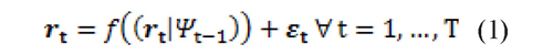
where ƒ (·) is an ARMA function and Ψt It is the set of information available at time t.
Furthermore, the conditional variance-covariance between the returns given by Eq. (2):

where Ht is a symmetric positive definite matrix.
Hence, if hij,t denotes the element of Ht and  it denotes the rth element of the returns t then the correlation between it and jt is given by Eq. (3):

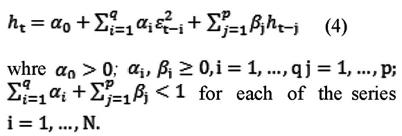
with ρij,t ∈ [-1,1] and each element of the diagonal of Ht follows a univariate GARCH process proposed by Engle (1982) and Bollerslev (1986), as follows:
Thus, the conditional variance-covariance matrix, Ht, can be written as follows:

where D. is the variance matrix and is equal to  and Pt is the matrix of dynamic conditional correlations.
The estimation of Ht is performed by the method of maximum likelihood in two stages: first, the conditional variance matrix is estimated; second, the conditional correlation matrix is estimated.
Once the dynamic conditional variance-covariance matrix is estimated it is possible to obtain standardized residuals that are equal to zt where:
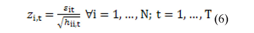
After obtaining the standardized residuals a pseudo sample is constructed for each series, in which the marginal distributions of the series are estimated using a semiparametric approach based on the EVT. This estimation of the marginal distributions also considers that financial series usually present distribution functions with heavy tails (another stylized fact of financial time series).
The pseudo sample is equal to:

Fi (·) is estimated semi parametrically: in the central part an empirical distribution function is estimated, and the EVT methodology, peaks over the threshold (POT), is used to estimate the parameters of the tails of the distribution (McNeil, et al., 2005).
The POT methodology suggests that the extreme observations, i.e, returns that are in the tails, follow a Generalized Pareto Distribution (GPD), as described in Eq. (8) (according to Fisher & Tippett (1928) and Gnedenko (1943)):
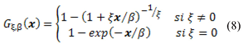
where β is a scale parameter, ξ a tail shape parameter and x = zi - νi where Zi are the standardized residuals obtained from Eq. (6) and νi is the chosen threshold. In the present study a threshold of 95 percent is used.
To determine whether the pseudo sample, ui fits the data properly the Kolmogorov-Smirnov (KS) statistic is calculated, which tests if ui distributes uniformly between zero and one.
Subsequently, we proceed to determine the dependency relationships between the series using copulas. Formally, a copula of dimension N is a distribution function in [0,1]N with standard uniform marginal distributions. Let (u) = C(u1,...uN) where C is a multivariate standard distribution function (dfs) that is a copula, then C: [0,1]N → [0,1] (McNeil, et al., 2005).
To understand the importance of copulas in the study of multivariate data is important to refer to the theorem of Sklar. This suggests that any multivariate distribution function contains copulas, and copulas can be used in conjunction with univariate dfs to build multivariate dfs (McNeil, et al., 2005). In other words, the theorem states that if F is the joint distribution function with margins F1,...,FN then there is a copula such that for all zi ∈ ℝ = [-∞,∞] i=1,...N, holds that:
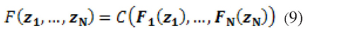
Thus if C(·) exists, this function contains all the dependence structure of the series.
In the present study, five types of multivariate copulas are used: Clayton, Gumbel, Frank, Normal and t-student.
To determine the copula that best fits the data we use four information criteria proposed by Joe (1997) and Zivot & Wang (2006) to compare between copulas. These criteria are: the logarithm of maximum likelihood, Akaike (AIC), Bayesian (BIC) and Hannan-Quinn (HQ). Which are defined as:
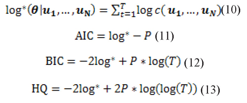
where θ is the vector of estimated parameters of the copula, c(u1,...,uN) is the density function of the copula, P is the number of estimated parameters and T is the number of data.
After selecting the best copula, m scenarios are simulated by means of the Monte Carlo technique based on the estimated parameters of the copula. The simulation gives as result the marginal distribution of each factor (ui), however by construction it is distributed uniformly between zero and one. Therefore we must perform the inverse operations of each step made to model the copulas, in order to obtain the marginal distribution of each factor in terms of returns.
This implies that the GDP inverse distribution function of the tails and the empirical distribution inverse of the marginal distributions must be obtained. In this process the marginal distributions of standardized returns, ri of the risk factors are obtained. These factors follow the same multivariate distribution.

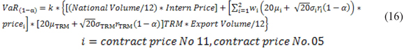
Finally, the VaR of the chosen output variable is calculated. This variable is affected by the risk factors simulated by means of copulas and EVT. The VaR is a method to model the uncertainty of the company, using statistical techniques to quantify the exposure to market risk that it faces.
Theoretically, the VaR is a measure of the maximum expected loss of a portfolio of assets in a given period, at a given confidence level α (Christoffersen, 2011). In the present study the portfolio is composed of the simulated returns ri Three risk factors are taken into account: the futures contracts price of the NY Stock Exchange (Contract No.11- raw sugar) and of the London Futures Exchange (Contract No.05 - white sugar) and the exchange rate between Colombian pesos and United States dollars (TRM for its acronym in Spanish). In addition, the gross profit is the output variable which is affected by the risk factors. The VaR of the gross profit is equal to:
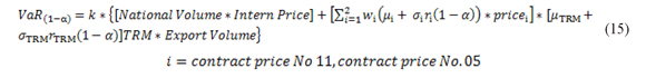
Where µi is the forecasted mean of the risk factor i for the next period, estimated using an ARIMA model. σi is the forecasted standard deviation of the factor i, estimated with a DCC-GARCH model. ri (1 - α) is the return located at position 1 -α of the loss distribution. wi is the proportion of sugar exports, raw or white, of total exports. Thus, the term

corresponds to the company's revenues from exports of sugar in the international market; revenues that are risky because they depend on the behavior of the three risk factors.
The term (National volume * Intern Price) corresponds to the company's revenues derived from domestic sugar sales, revenues that are risk- free as the price received by the sugar mills is regulated by the Sugar Price Stabilization Fund (FEPA for its acronym in Spanish). FEPA is an instrument that operates as a clearing house, managed by Asocaña. The stabilization fund charges producers and exporters who sell the sugar on the market at a price above the reference price of the FEPA. By contrast, the fund pays a (Contract No.11- raw sugar) and of the London Futures Exchange (Contract No.05 - white sugar) and the exchange rate between Colombian pesos and United States dollars (TRM for its acronym in Spanish). In addition, the gross profit is the output variable which is affected by the risk factors. The VaR of the gross profit is equal to:
Pricesi is the price of the last day of the risk factor i series. µTRM is the TRM forecasted mean for the next period. σTRM is the TRM forecasted standard deviation. rTRM (1 - α) is equal to the TRM return located at position 1 - α of the loss distribution. TRM is the value of the exchange rate on the last day of the series.
compensation when the market price is lower than its reference price.
Finally, k is the ratio [1 - (Sales Costs/Operational Revenues)]
As risk factors have a daily frequency, the VaR of the company's gross profit calculated is on a daily basis. To obtain the VaR on a monthly basis (the enterprises' profits are consolidated monthly) it is necessary to divide the volume of domestic sales and exports between 12. Also, following Melo & Granados (2011), we must multiply the forecasted mean by 20 and the forecasted standard deviation by √20 Hence, the monthly VaR of the gross profit is equal to:
3. Results and discussion
As mentioned in the previous section, the three risk factors simulated are the futures contract price No. 05 of the London Futures Exchange (LIFFE), the futures contract price No. 11 of the New York Stock Exchange in the Intercontinental Exchange (ICE) and the TRM. The frequency of the data is daily and the period of analysis is from January 3 of 2003 until February 28 of 2014.
The contract No. 05 is the world benchmark contract for the sales of white sugar. The contract provides a price for physical delivery of 50 tons of raw sugar, FOB-port of shipment. The contract No. 11 is the world benchmark contract for the sales of raw sugar. The contract provides a price for physical delivery of 112,000 pounds of raw sugar, FOB-port of shipment.
The prices of the three risk factors are presented infigure 1. The three series are possibly non- stationary in mean, since the series do not fluctuate around their average value. In addition, the series present trends. Therefore, it is necessary to perform unit root tests to determine the order of integration of the series, and to determine if it is necessary to differentiate in order to make them stationary in mean.
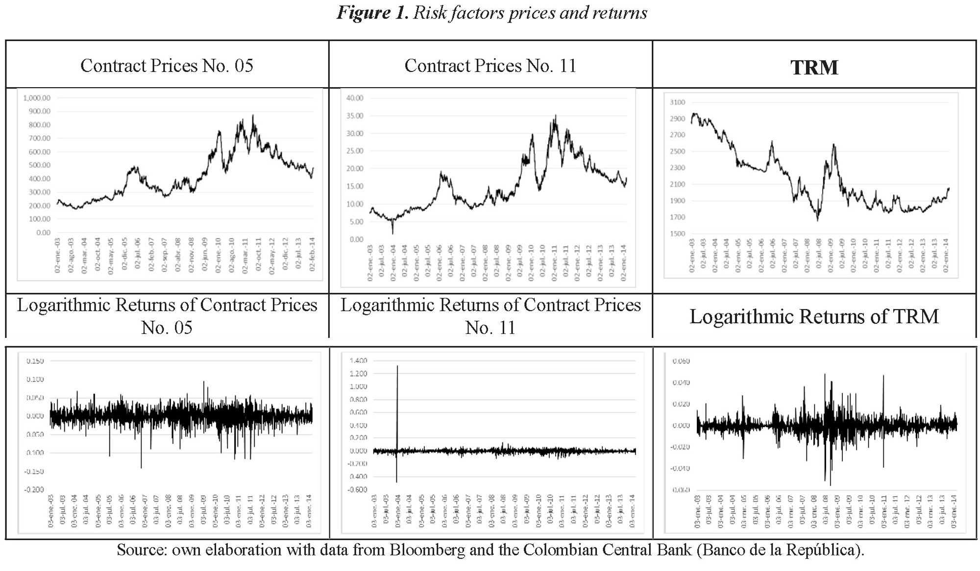
Additionally, in Figure 1 the price returns of the three risk factors considered in this study are presented. In the figures we can see that the series might present some stylized facts of financial series such as volatility clusters and heteroskedasticity.
Because the series in levels present signs of nonstationarity in mean, a Dickey-Fuller test was performed for each of them. Three test versions were performed: the first determines whether the series presents a unit root, this is done with the series in levels and without including intercept or trend; the second determines if the series is trend stationarity, in this case an intercept and a trend component is included; the third test is performed to determine whether the series has a stochastic trend or not.
Given the results of the tests, it can be concluded that the three series have a stochastic trend component, then it is necessary to differentiate the series to make them stationary in mean. Once the series are differentiated we proceeded to model the series in mean by an ARIMA model. For the series of prices No. 05 an ARIMA (1,1,1) was chosen and the forecast of the returns' mean is 0.000295. For the series of prices No. 11 an ARIMA (3,1,2) was selected and the forecast of the returns' mean is 0.000286. For the TRM series an ARIMA (1,1,0) was chosen and the forecast of the returns' mean is -0.000118.
Subsequently, the variance of each series was model by means of a DCC-GARCH model, and the filtered residual series obtained. The pseudo sample was constructed using the filtered residuals, where the tails are adjusted to a Generalized Pareto Distribution, and the center follows an empirical distribution. The EVT parameters of scale and shape of each distribution and the statistic KS are presented in Table 1.
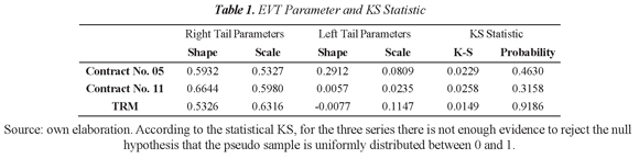
Table 2 shows the parameters of the estimated copulas and the selection criteria. The copula that best fits the data is the t-student, it presents the maximum likelihood and AIC, and minimizes the BIC and HQ criteria.
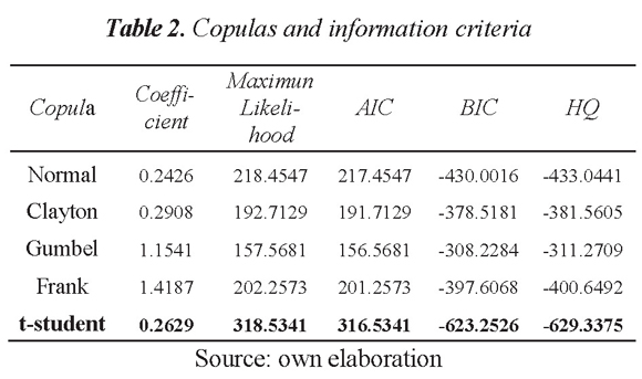
After choosing the t-student as the copula that best describes the dependency relationships between the three risk factors, 1,000 scenarios were simulated using the Monte Carlo technique based on the estimated copula's parameters. The marginal distribution of each factor was obtained from the simulation.
The standardized distributions of the risk factors' marginal returns, , that follow the same multivariate distribution were obtained after performing the inverse operations of the steps made to model the copulas.
With the standardized residuals and hypothetical information from a sugar mill that produces raw and white sugar, the VaR of the monthly average gross profit was constructed at 95% confidence. The sugar mill hypothetical values are presented in Table 3.
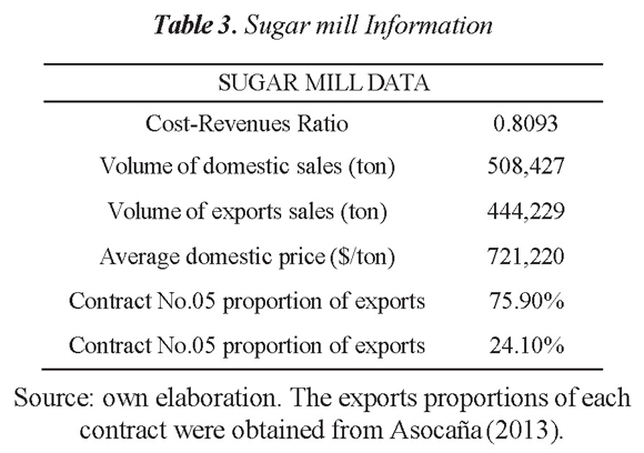
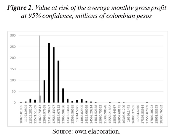
According to these values and the estimates, the value at risk of the average monthly gross profit at 95% confidence is equal to $ 11,758,951,371 Colombian pesos (COP). That is, with a 95% confidence level the company can expected to have a minimum of $ 11,758,951,371 COP monthly gross profit.
Figure 2 presents the histogram of the loss function estimated, as the calculated VaR.
Finally, the utility at risk calculated is compared with the operational expenses of the company. The monthly fixed costs are $ 6,383,767,000 COP, so the company can expect to be above the break-even point in terms of revenues.
4. Conclusions
The present study performed an application of a methodology for optimal selection of investment projects. This methodology suggests that optimal management of uncertainty requires the identification and quantification of companies' risk exposures through appropriate econometric techniques. Among the econometric techniques applied are: ARIMA models for forecasting risk factors; modeling autoregressive conditional volatility of the risk factors; EVT application for modeling the tails of the factors' distribution factors; multivariate modeling of dependency relationships between series by copulas.
The application of this methodology in a hypothetical company of the sugar sector allowed modeling three risk factors that affect its gross profit. These risk factors are the prices of sugar futures contract 11 and 5, and the TRM. To model the multivariate dependence between the risk factors, for each series its mean and variance were modeled using ARIMA processes and DCC- GARCH models. Subsequently, a pseudo sample was constructed by EVT to adequately model the tails of the distribution that are of special interest in financial series. We proceeded to estimate different copulas to determine the one that best fits to the data, this was the t-student copula. Then, 1,000 scenarios were simulated using Monte Carlo techniques based on the parameters estimated of the copula selected. However, the distributions simulated by construction are distributed between zero and one, therefore the inverse operations of each step were performed to obtain the marginal distribution of each factor in terms of returns.
Afterwards, we estimated the value at risk of operational gross profit, output variable that is affected by the risk factors modeled. In this case, the factors do not affect the total gross profit, they affect only the part derived from exports. For the sugar mill a volume of domestic sales and exports were supposed to estimate the VaR. The value at risk of the average monthly gross profit at 95% confidence is equal to $ 11,758,951,371 COP. In addition, the utility at risk calculated was compared with the operational expenses of the company, concluding that it can expect to be above the break-even point in terms of revenues.
The above results are important inputs for subsequent valuations of specific investment projects in a much more robust manner than traditionally done. Although the methodology used in this study faces many of the shortcomings in traditional assessment strategies of investment projects, the methodology does not take into account that risk scenarios that companies face may vary over time, i.e, they may be dependent on the state. In the case of companies that export, e.g, face macroeconomic risks such as exchange rate and commodity prices. These risks behave differently, for example, in times of drought and no drought in the places of production of the good. Listed security companies are another example; they face the market risk arising from the exposure of their portfolios to the price of various stock indices. These indices evolve differently according to economic booms and recessions.
Due to the above considerations it is relevant for future research to advance theoretically and empirically in the understanding of the risk factors that affect companies, in particular it is desirable to expand the understanding of the dynamics underlying the different ways of measuring risk across different regimes.
5. Aknowledgements
I want to thank the Colciencias Program "Jóvenes Investigadores e Innovadores Virginia Gutiérrez de Pineda" and the Universidad del Valle for financial support. I also thank Professor Diego Fernando Manotas, Professor Jorge Mario Uribe and Professor Ines Maria Ulloa for their valuable guidance and support during the making of this document. Finally, I thank the members of the research group Applied Macroeconomics and Financial Economics, especially Natalia Restrepo and Julian Fernandez for their comments and feedback.
6. Bibliographic references
Asocaña (Association of Sugarcane Producers of Colombia). (2013). Aspectos Generales del Sector Azucarero 2013-2014. Cali, Colombia: Asocaña. [ Links ]
Bollerslev, T. (1986). Generalized Autoregressive Conditional Heteroskedasticity. Journal of Econometrics, 31 (3), 307-327. [ Links ]
Chevallier, J. (2011). Detecting instability in the volatility of carbon prices. Energy Economics, 33 (1), 99-110. [ Links ]
Christoffersen, P. (2011). Elements of Financial Risk Management (2 ed.). Waltham (MA), USA: Academic Press. [ Links ]
Cifter, A. (2013). Forecasting electricity price volatility with the Markov-switching GARCH model: Evidence from the Nordic electric power market. Electric Power Systems Research, 102, 61-67. [ Links ]
Engle, R. (1982). Autoregressive Conditional Heteroskedasticity with Estimates of the Variance of United Kingdom Inflation. Econometrica, 50 (4), 987-1007. [ Links ]
Engle, R. (2002). Dynamic Conditional Correlation: A Simple Class of Multivariate Generalized Autoregressive Conditional Heteroskedasticity Models. Journal of Business & Economics Statistics, 20 (3), 339-350. [ Links ]
Feng, Z. H., Zou, L. Le., & Wei, Y. M. (2011). Carbon price volatility: Evidence from EU ETS. Applied Energy, 88 (3), 590-598. [ Links ]
Feng, Z.-H., Wei, Y.-M., & Wang, K. (2012). Estimating risk for the carbon market via extreme value theory: An empirical analysis of the EU ETS. Applied Energy, 99, 97-108. [ Links ]
Fisher, R., & Tippett, L. (1928). Limiting Forms of the Frequency Distribution of the Largest or Smallest members of a Sample. Proceeding of the Cambridge Philosophical Society, 24 (2), 180-190. [ Links ]
Gnedenko, B. (1943). Sur La Distribution Limite du Terme Maximun D'une Serie Aleatorie. Annals of Mathematics, 44 (3), 423-453. [ Links ]
Hai, X., & Yang, B. (2014). Research on the risk measurement of EU carbon market based on VaR-GARCH models. WIT Transactions on Information and Communication Technologies, 52, 1259-1264. [ Links ]
Joe, H. (1997). Multivariate Models and Dependence Concepts. London, UK: Cahpman & Hall. [ Links ]
Manotas, D. F. (2009). Optimal Economic Project Selection under Uncertainty: An Illustration from an Utility Company. Ingeniería y Competitividad, 11 (2), 41-52. [ Links ]
Manotas, D.F., y Toro, H. H. (2009). Análisis de decisiones de inversión utilizando el criterio valor presente neto en riesgo (VPN en riesgo). Revista Facultad de Ingenieria Universidad de Antioquia, 49, 199-213. [ Links ]
McNeil, A., Frey, R., & Embrechts, P. (2005). Quantitative Risk Management: Concepts, Techniques, and Tools. New Jersey, USA: Princeton University Press. [ Links ]
Melo, L.F., y Granados, J.C. (2011). Regulación y Valor en Riesgo. Ensayos sobre Política Económica, 29 (64), 110-177. [ Links ]
Uribe, J. M., Ulloa, I. M., & Manotas, D. F. (2015). A Methodological Proposal to Incorporate Market Risk into Real Sector Financial Projections. Mimeo. Cali, Colombia, Universidad del Valle. [ Links ]
Wang, H., He, K., & Zou, Y. (2014). EMD Based Value at Risk Estimate Algorithm for Electricity Markets. In, Proceedings of the 2014 Seventh International Joint Conference on Computational Sciences and Optimization (pp. 445-449) Beijing, China. [ Links ]
Wang, J., & Wang, R. (2014). Evaluating electricity price volatility risk in competitive environment based on ARMAX-GARCHSK- EVT model. International Journal of Computer Applications in Technology, 50 (3/4), 174-179. [ Links ]
Xiong, S. F., & Zou, X. Y. (2014). Value at risk and price volatility forecasting in electricity market: A literature review. Power System Protection and Control, 42 (2), 146-153. [ Links ]
Yang, J., & Lin, P. (2011). Dynamic risk measurement of futures based on wavelet theory. In, Proceedings of the 2011 Seventh International Conference on Computational Intelligence and Security (pp. 1484-1487). Sanya, Hainan Province, China. [ Links ]
Zhang, C., Yang, Y., & Zhang, T. (2013). The integrated measurement of carbon finance market risk based on Copula model. In, Proceedings of the 4th International Conference on Risk Analysis and Crisis Response (pp. 561-566). Istanbul, Turkey. [ Links ]
Zivot, E., & Wang, J. (2006). Modeling Financial Time Series with S-Plus®. New York, USA: Springer. [ Links ]

Revista Ingeniería y Competitividad por Universidad del Valle se encuentra bajo una licencia Creative Commons Reconocimiento
