1. Introduction

Reliability is defined by Dhillon ¹ and Nachlas ² as the probability that an article will perform the assignment satisfactorily over a period of time, when it is used according to specified conditions, identifying four factors: probability, proper functioning, environment and time. Dhillon ¹ adds that many mathematical definitions and probabilistic distributions are used to perform different types of reliability studies.

Nachlas ² and Mitra ³ argue that the distribution function that is most often used to model reliability is that of Exponential distribution; on other occasions different theoretical distributions are used, such as the Weibull or the Gamma. They add that for the statistical methods of reliability estimation, whether parametric or non-parametric, the failure data obtained during the life tests of the components are used. Regarding the calculation of confidence intervals, in Kundu & Basu ⁴ it is argued that the best results are obtained through the Exponential and Weibull distributions. Other authors, such as Percontini ⁵ make new distribution proposals, such as ZETA-G. However, Wang & Pham ⁶ point out that in practice many systems are complex, they can follow different failure distributions and many times there is not sufficient failure data, therefore it is impossible to obtain the confidence intervals for the different reliability indexes. According to Makhdoom & Nasiri ⁷, many researchers are unable to observe the life cycle of the tested units due to a lack of time, resources, or problems with data collection; the sample is therefore truncated, resulting in different types of errors. Mitra ³ states that the study of the life cycle of elements is important in many aspects, the primary interest being to find out the distribution that supports the data collected.

It should be noted that failure data obtained during component life tests are carried out by hurried and costly methods, in which environmental conditions cannot always be fully emulated. Therefore, obtaining the minimum amount of data needed to perform the calculations under real operating conditions is extremely difficult, since you have to observe the events naturally as they occur during the operation of the machines. This situation causes many difficulties when trying to obtain an adequate minimum sample size of failures, as it is necessary to wait for years of operation, making it impossible to carry out the investigations since they will not be valid or the equipment will have already aged and / or will be obsolete.

It has been proven that the Monte Carlo technique combined with other methods is a powerful tool for dealing with this type of problem; Wang & Pham ⁶. Since the 1940s, tools have been developed to simulate the occurrence of events. To date, the most popular and widely used has been the Monte Carlo method in some of its variants: crude, stratified, by complements and others; Lieberman & Hillier ⁸. This situation explains why, in many cases, reliability studies to adjust maintenance plans are not performed. In other words, it is very unlikely that in the production processes, reliability studies will be carried out. This may be due to different causes, such as:

Maintenance management is poor, with the consequence of failing to log and monitor the occurrence of the failures; the data recorded is not reliable; engineering staff do not have sufficient knowledge or skill to deal with statistical techniques, or do not know how to use the computer tools that currently exist.

In many entities and branches of the economy there is a poor understanding of how important these studies can be to improve or perfect the functionality, safety and durability of machinery; in other words, operational reliability.

Finally, some data is sometimes available, but due to its scarcity (the number of elements in the sample not being sufficient), it does not allow for the calculation and research required. To solve the problem of not having the sample size needed to estimate the necessary parameters, several algorithms are proposed, supported by the Monte Carlo simulation method, Wang & Pham ⁶. These numerical methods allow the solution of different types of problems by means of probabilistic systems models and the simulation of random variables. It is worth highlighting that in other studies, Paz-Sabogal et al. ⁹, there is an assumption that the theoretical distributions of failure are known, as is the case with Lognormal and Weibull, a situation that is generally unknown at the actual stage of operation and maintenance of the machines.

The work of Ramírez et al. ¹⁰ demonstrates how difficult it is to determine the minimum sample size and the number of bootstrap samples to be used to obtain appropriate sample distributions; for said study, the simulation of the samples was obtained through the Gamma distribution. According to Efron & Tibshirani ¹¹, the term bootstrap could be interpreted as "To advance by one's own effort", "To multiply one’s experiences from those already lived". It is no more than a method of re-sampling data, i.e., from an original sample the same one is replicated several times, Ledesma ¹². According to Edwards et al. ¹³, it is of particular interest to estimate percentiles in reliability studies and the study argues that when sample sizes are sufficiently large, reasonable approximations are obtained, but not for cases where the sample is insufficient and it states that the fundamental idea behind the use of bootstrap is that the empirical distribution thus obtained provides an approximation to the theoretical sample distribution of interest. However, Christopher et al. ¹⁴ suggest that bootstrapping is an ambiguous statistical method, since in most applications the methodology leaves the researcher with two types of errors: those originated by the initial data set and those generated by the re-sampling system, and therefore propose a method to eliminate re-sampling errors. In the processes of operation and maintenance of the machines, under environmental conditions that were not considered by the manufacturer, two real problems arise:

The functions of the components’ and subsystems’ joint distribution of failure are unknown.

Failure data is insufficient to estimate confidence intervals for different reliability indices necessary to adjust and refine maintenance plans for machines and installations.

Taking into account these difficulties, the present work proposes a methodology based on the Monte Carlo and bootstrap method that would allow to obtain the function of failure distribution of the machines and with it enable the calculation of the confidence intervals for different reliability indices and thus enable the readjustment of the maintenance plans in real time, in accordance with the technical state of the machinery.

2. Methodology

The need to carry out research within a given time period and not having, for the sample being studied, sufficient data that allows to make up a representative sample, is a common occurrence in the daily life of the researcher, so it is necessary to simulate such data under the conditions in which the probabilistic distribution of the sample is unknown. For the new simulated data to be representative of the elements to which the sample belongs, the authors of this work propose the following procedure:

Define and delimit the sample space or universe (U) where the phenomena or events that will be studied occur.

Register a minimum amount of data regarding the phenomenon that conform to the sample elements. With a bigger sample size, the results will be better. It is worth highlighting that this is the problem that one trying to solve, because the reality is that the sample often does not exceed 5 or 6 elements.

With the data observed, the interpolation process is carried out to obtain a continuous function f(x).

The empirical probability of the occurrence of the events is determined as the ratio between the number of type A events that happened and the total number of observed events. The occurrence of the events is considered completely random. It is necessary to clarify that this process can be carried out with the original data or with data calculated from the function and interpolation already obtained.

(1)

With the calculated probabilities, a new interpolation process is carried out with which an accumulated continual probabilistic distribution p(x) is able to be obtained.

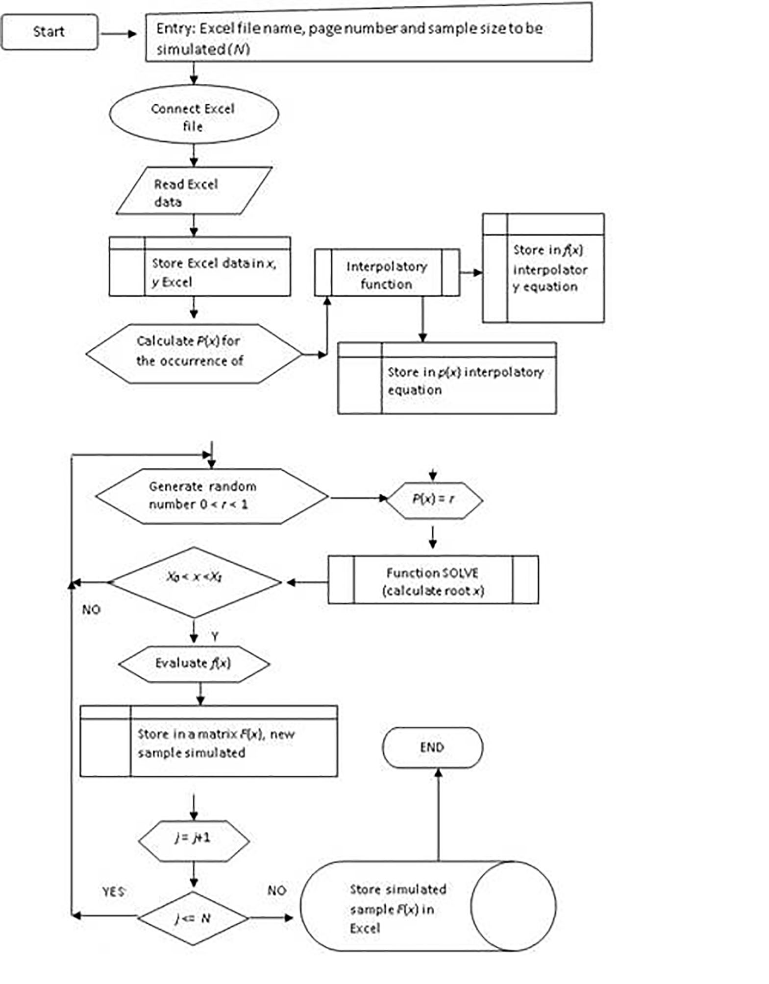
Supported by the crude Monte Carlos method, random numbers n _i between 0 and 1 are generated, for each n _i the equation p(x) = n _i is set out and resolved with the objective of obtaining the value of the corresponding pre-image x.

In obtaining a value for the pre-image x, this is then evaluated in the function f(x), thereby revealing a new simulated figure which will become the elements that make up the population sample that is needed to define the probabilistic density function necessary to find out which type of theoretical distribution the data resembles most.

Once the theoretical distribution is known, said data is used to carry out the calculations appropriate to the problem to be solved.

3. Results and discussion

3.1. Example of the application of the aforementioned algorithm

It is necessary to perform a study of the Gamma Resource durability index (T(()) of a determined mechanical element E ₁ , which in turn belongs to a more general system S, which contains other mechanical elements denoted as E ₂ , E ₃ ,...., E _n-1 , E _n . The system S belongs to a population of machines.

To calculate the Gamma Resource (Gamma distribution Lifespan) T(() of element E _1, it is necessary to look at the statistics relating to its central tendency and dispersion: its mean-time to failure, the standard deviation and the gamma percentile. To carry out the calculations of said statistics it is necessary that the machine element E ₁ has failed enough times that the sample made up of said events is representative of its population (u). As the number of working hours necessary for element E ₁ to fail is relatively large, a period of time would be needed that is too long to carry out a study of the Gamma Resource durability index of this machine element. The solution used in practice is to simply do without said study as its completion turns out to be impossible.

To seek and encounter an investigative alternative it is necessary to apply the procedure describe in this work.

The sample space or universe (U) is defined and delimited as that made up of all of the possible ways in which element E ₁ could fail during the life-cycle of the range of machines available in the country. Due to the nature of this phenomenon it can be confirmed that the sample space is infinite.

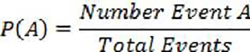
The failures of element E ₁ are registered. For the particular case studied, the working hours of the machines sampled is given as the mean-times until the failure: 120, 250, 267, 320. The data is shown in Table 1 for the purpose of interpolation and identification of the analytical function f(x).

Table 1 Accumulated working hours of the machine and duration until element failure E1 

Variable	Machine working hours
X	0	120	370	637	957
Y	0	120	250	267	320

With the data observed in point 2 the interpolation process is carried out, obtaining the continuous function (equation 2), which is represented in Figure 1.

(2)

Figure 1 Continuous interpolation function f(x). 

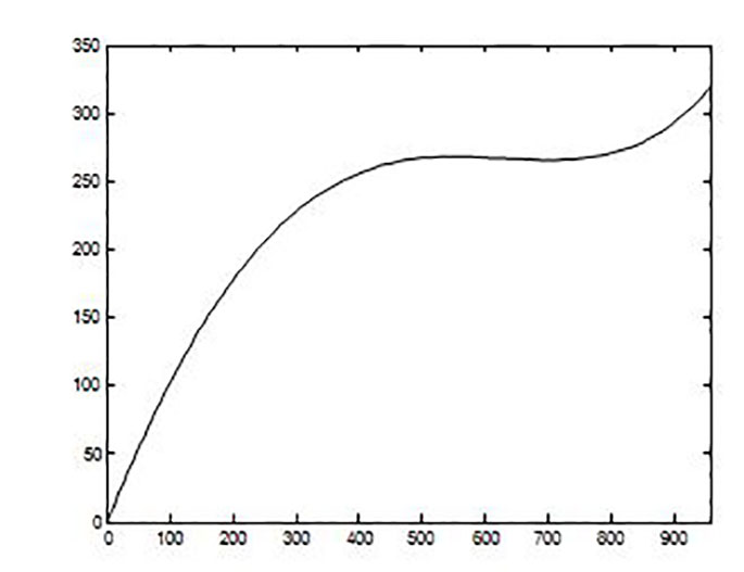
The empirical probability of occurrence of the events is determined as the ratio between the number of accumulated hours in which the failure of element E ₁ occurred and the total accumulated hours observed, as shown in Table 2. As can be seen, for convenience of calculation, the table shows the empirical probabilities of the original data. However, any value of failure time can be obtained by evaluating for the number of hours worked in Eq. (3), thereby calculating the empirical probability of occurrence of the failure.

Table 2 Empirical probabilities of element failure E1. 

Variable / function	Machine working hours
X (Independent)	0	120	370	637	957
P(X) (Values obtained from the probabilistic function)	0	0.1254	0.3866	0.6656	1.000

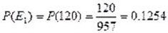(3)

With the probabilities calculated in step 4, a new interpolation process is performed to obtain a continuous probabilistic function p(x), represented graphically in Figure 2.

Figure 2 Function of probabilistic empirical distribution p(x). 

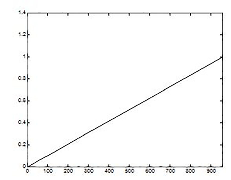
(4)

Supported by the Lieberman & Hillier (8) Monte Carlo method, the random numbers n _i are generated between 0 and 1, for each n _i one poses and solves the equation p(x) = n _i to obtain the value of the corresponding Pre-image x. Using the MATLAB application, the random number 0.2311 was generated with the "rand" function, which is equal to the probabilistic function obtained in step 5 and from this equation, the possible roots are calculated by any of the classical numerical methods:

The pre-image calculated is x ( 221.1653.

The found value of pre-image x is evaluated in the function ((x), finding a new simulated data (mean time between failures of element E1). All of the above steps are developed with the help of the block diagram shown in Figure 3, which was programmed with the mathematical assistant MATLAB.

Figure 3 Calculation algorithm. 

The investigated reliability index, i.e. the Gamma lifetime, also called Gamma Resource, is calculated in a 90% confidence interval with the simulated data shown in Table 3.

Table 3 Example of a simulated sample of 100 elements. 

simulated sample
172	272	266	248	238	268	211	217	269	267
268	268	258	274	219	261	202	264	266	62
211	174	225	273	238	266	277	67	268	268
172	267	166	268	268	268	266	314	268	53
17	271	169	266	266	267	129	269	178	256
266	21	267	282	227	300	13	257	248	225
261	267	224	269	271	267	281	267	267	277
291	248	268	268	269	278	172	235	267	16
263	270	140	269	246	155	223	259	263	266
257	266	266	267	266	310	267	188	269	306

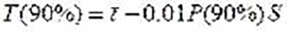(5)

Hours

Where

ῑ = 235.2 - Mean time between failures

S= 65.7 - Standard deviation

P = 276.7 - Percentile for 90% confidence

The proposed procedure allows the realization of the number of replicates required and to be able to estimate the parameters of the probabilistic distribution function that represent the data initially collected and thus calculate the necessary statistics that will allow performing the required calculations. In the particular case of the study shown, a hundred data were generated, which are shown in Table 3 and, when processed, the mean time between failure, the standard deviation and the percentile needed to calculate the reliability index of the gamma life was obtained.

With the data obtained, other reliability indicators might be calculated, such as the probability of working without system failure up to a pre-established number of hours. The proposed procedure is easy to program, based on the block diagram provided in this work. In order to evaluate the possible errors of estimation of the calculated statistics the methodology proposed in the work by Ramírez et al. (10) is suggested. On the other hand, the authors insinuate to find news methodologies to evaluate the possible errors of estimation of the calculate statistics.

4. Conclusions

With the proposed procedure, we can simulate the data of a sample so that it is representative of its population size and from the obtained values, the parameters for the studied population can be inferred.

In addition, this makes it possible to carry out the necessary calculations of the research task in particular.