1. Introduction

The temperature integral (Equation 1) is,

(also named Arrhenius integral) is used in many non-linear analysis regression methods of thermogravimetric data as the solution of the differential equation that represents the variation in time of the fractional extent of conversion, or its integration between consecutive values ^1-3. In the field of thermal analysis most integral results are based on some approximate representation of 𝑝(𝑥) (general-purpose mathematical software, for example spreadsheets, do not include the temperature integral). But despite their prevalence in thermal analysis these approximations are in fact not necessary: 𝑝(𝑥) and its generalized form 𝑝_𝑚(𝑥) can be calculated with specific series representations, and more importantly they can be rewritten in terms of the special functions ⁴.

Thermogravimetric analysis (TGA) has become a common technique for chemisorption, thermal decomposition, and solid-gas reactions. For the most part analysis of thermogravimetric data is settled in the ICTAC Kinetics Committee recommendations ^5,6; but it is still an active research area and new methods have appeared after the ICTAC publications ^7-9. There are also some aspects of TGA data analysis, such as heat inertia, still under development ^10,11; while some others, like the use of logistic equation have been criticized ¹². In our previous work both the prevalence of the linear regression and the use of approximations to 𝑝(𝑥) were rebutted developing a non-linear regression method for thermal analysis data based on the general form of the temperature integral ⁴.

In this explanatory work we focus solely on the calculation of 𝑝_𝑚(𝑥) with special functions, starting with the development of a rigorous integration method to obtain benchmark values of the temperature integral for any value of 𝑚 or 𝑥. This required two related tasks explained in Section 3, first a tiny stepsize was chosen minimizing the error associated to the integration method; and second, and an algorithmic equivalent of the infinity upper limit was established. Next, in Section 4, an overview of available direct representations of 𝑝(𝑥) in power series is presented followed by the transformation of 𝑝_𝑚(𝑥) into special functions. Finally, the choice of the incomplete gamma function (Γ) is jusjpgied by comparisons against the numerical integration results. This conclusion is relevant not only for data analysis but also for the testing or calibration of the software built in, or included with, TGA instruments which is proprietary and tends to operate as a black box.

2. Generalization of the temperature integral

In thermal kinetics the fractional extent of conversion (α) is usually written as the product of the Arrhenius rate constant and a kinetic function 𝑓 (Equation 2):

Where 𝑅 is the ideal gas constant, and the activation energy 𝐸 is also constant. But in some variants of this model the preexponential factor is a function of temperature in the form of the Equation 3:

Where 𝐴₀ is a constant ¹³. Integration of Eq. (2) with a constant heating rate 𝛽 leads to Equation 4

Where Equation 5 is the general form of the temperature integral, being 𝑝 a particular case of 𝑝_𝑚 with 𝑚=0 and 𝐴=𝐴₀.

The integration variable χ is dimensionless, and the temperature defines the lower limit 𝑥=𝐸/𝑅𝛵, but it implies that the limit 𝛵₀→0 becomes 𝑥→∞. This indeterminate limit does not allow an analytical solution, but at the same time relates 𝑝_𝑚 with the special functions, as it will be explained in Section 4. On the other hand, the upper infinity limit is certainly an issue for the numerical integration of 𝑝_𝑚, but it is solved in the next section.

For the comparisons between 𝑝_𝑚 values from formulas and from numerical integration in the following sections we chose 𝑚= −3, −2.5, …,0, …,3 because values of 𝑚 between -1.5 and 2.5 in 0.5 increments have been reported for solid decomposition and gas-solid reactions ¹³. It is true that temperature-dependent preexponential factors are much less common than constant 𝐴s, but our analysis of the general temperature integral covers 𝑝(𝑥) as the particular case 𝑚= 0, and 𝐴 = 𝐴₀. Lower limit values were set as 𝑥=1,2,5…,100 because 𝑥 values in the interval [5,100] have been considered of practical significance ¹⁴.

3. Numerical integration

There are no sources of exact values for 𝑝_𝑚(𝑥), it does not have analytical solution and even the tables for 𝑝(𝑥) are rare, for example the Vallet compilation was published last in 1961 ^1,15,16. However 𝑝(𝑥) reference values have been obtained by means of numerical integration, with the trapezoidal rule, or the integration routine included in the software Mathematica ^17-20.

In this work the reference values were also calculated by numerical integration the with the Simpson 3/8 rule. It was chosen as a compromise between accuracy and efficiency, after considering that for the same stepsize (ℎ) the most intricate methods offer a better accuracy than the simple ones, but given that accuracy is inversely proportional to the stepsize, even simple methods can produce a very low error using a tiny ℎ.

Following the Simpson 3/8 rule the temperature integral is approximated as the area sum (Equation 6):

Where each term is calculated in a subinterval of length 3ℎ with the Equation 7:

Evaluating the argument of the integral, 𝑓(χ), at the points χ_0𝑖, = 𝑥 + 3(𝑖 −1)ℎ, χ_1,𝑖, = χ_0,𝑖+ℎ, χ_2,𝑖, = χ_0,𝑖+2ℎ, and χ_3,𝑖, = χ_0,𝑖+3ℎ ^21,22.

It was also necessary to define the value of h, but the only guideline found in the literature was a temperature stepsize of 10⁻²K, which is useless as the integration variable is 𝑥 = 𝐸/𝑅𝛵, not 𝛵 ¹⁹. In order to choose a stepsize 𝑝_𝑚𝑠 obtained with ℎ values from 1 down to 10^-5 were probed, finding that the averaged relative difference (Figure 1) is less than 1% for any stepsize ℎ<1, and that the avgs were almost the same for ℎ = 10⁻⁴ and ℎ = 10⁻³. Although these results suggest that a stepsize of 0.001 is enough the reference values of 𝑝_𝑚(𝑥) were calculated with a stricter value of ℎ = 10⁻⁵, which is much smaller than typical values of χ. The associated error in the Simpson 3/8 rule is │(3ℎ⁵/80)𝑓⁽⁴⁾(ξ)│ =3.75( 10⁻²⁷(│𝑓⁽⁴⁾(ξ)│, where ξ is a value between the limits of integration ²².

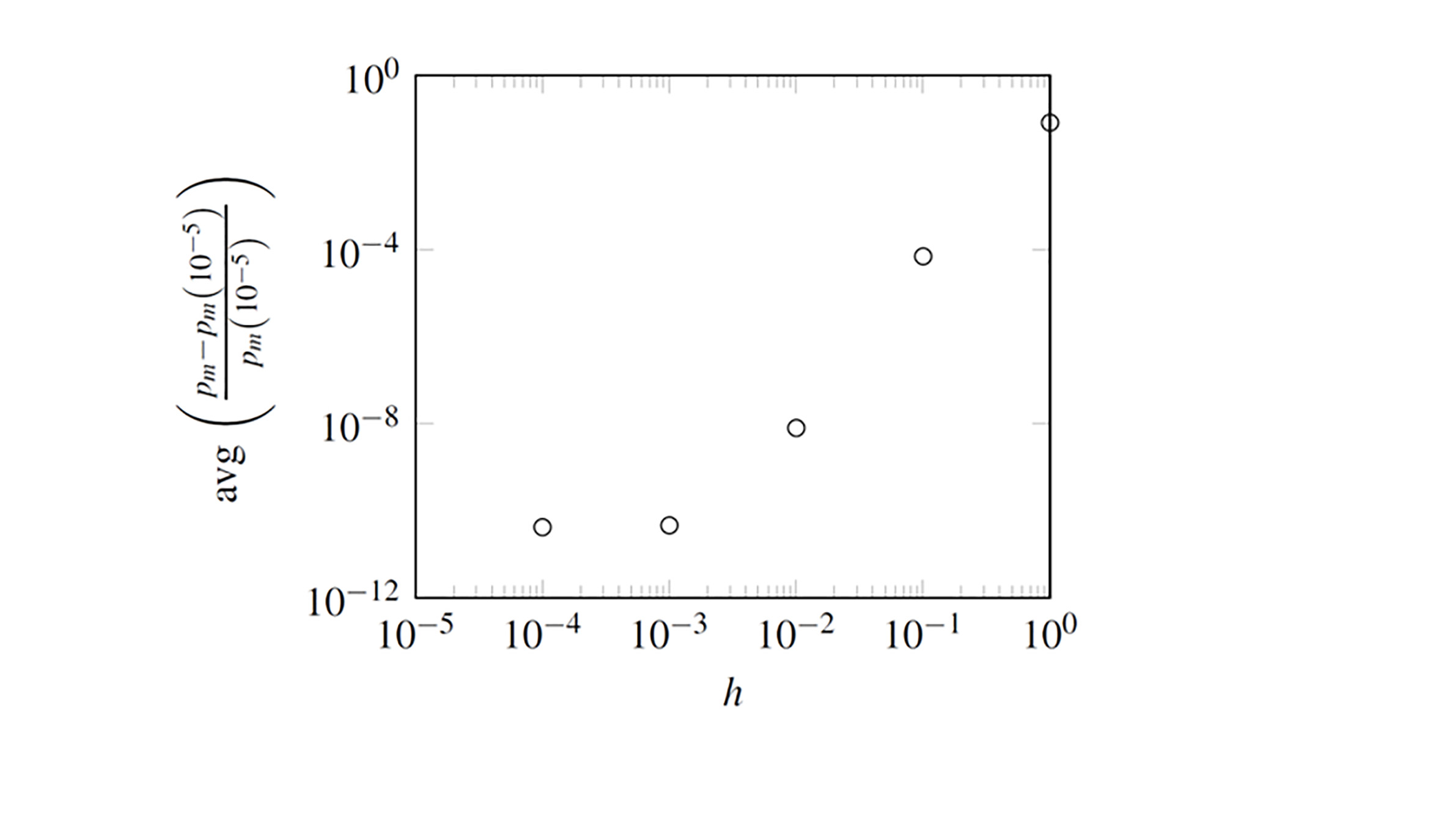
Figure 1 Averaged relative difference in 𝑝_𝑚(𝑥) values respect to the reference result with h = 10⁻⁵ (own source) 

Another issue in the numerical integration of Equations 1 and 5 arises from the representation of their infinity upper limits with some finite value, namely 𝑥_∞. An apparently obvious choice for 𝑥_∞ is the biggest possible real number in the system, 1.79(10³⁰⁸ in the double precision 64 bit IEEE 754 standard ^23-25, but it would require an unbearable long calculation time (a back of the envelope estimation for integration with the trapezoidal rule using ℎ = 1 and 1𝜇𝑠 per step yields 3 (10²⁹⁴ years).

It was also considered defining 𝑥_∞ as the value such where the argument of the integral vanishes, that is 𝑓(𝑥_∞) ≈ 0 ≈ σ, where σ is the tiniest possible real number in the system (σ = 4.94(10⁻³²⁴ for double precision variables, standard IEEE 754). In this way, Equation 8:

And the results of solving this equation for −3 ≤ 𝑚 ≤ 3 lead to 𝑥_∞=750. However, this hypothetical upper limit choice is computationally wasteful because for most of the 𝐴_𝑖 terms in Equation 6 the addition is irrelevant and unfeasible. It is illustrated here with an extreme example: using ℎ = 10⁻⁵ and 𝑚= −3 the result is 𝑝₋₃(100) = 3.76(10⁻⁴², but the value of 𝐴_𝑖(χ = 600) is 4.77 ( 10⁻²⁶³, and the following 𝐴_𝑖𝑠 are even smaller.

Due to the order of magnitude difference, 10⁻⁴² vs. 10⁻²⁶³, the addition of 𝐴_𝑖(χ = 600) and the following 𝐴_𝑖𝑠 s does not alter the resulting value of 𝑝_𝑚, it would only change its 221th and following digits, which are irrelevant in the sum. Moreover, these hundreds of digits do not exist, and are unnecessary, because the calculations of TGA data analysis is carried out with standard real variables of 15-17 decimal digits, which provide enough precision for the estimation of parameters (we emphasize that hypothetical number representations with hundreds of digits are not necessary for TGA data analysis).

A static upper limit 𝑥_∞ was discarded after considering the reasons in the previous paragraph, but Figure 2 shows that the integral argument in 𝑝_𝑚(𝑥) decreases asymptotically to 0, suggesting to use the point where it becomes negligible as an equivalent to 𝑥_∞. In this way the area sum of Equation 6 is stopped in a dominant term, idenjpgied with the index 𝑖_∞ such that the subsequent terms do not numerically add to the result. Given that

And

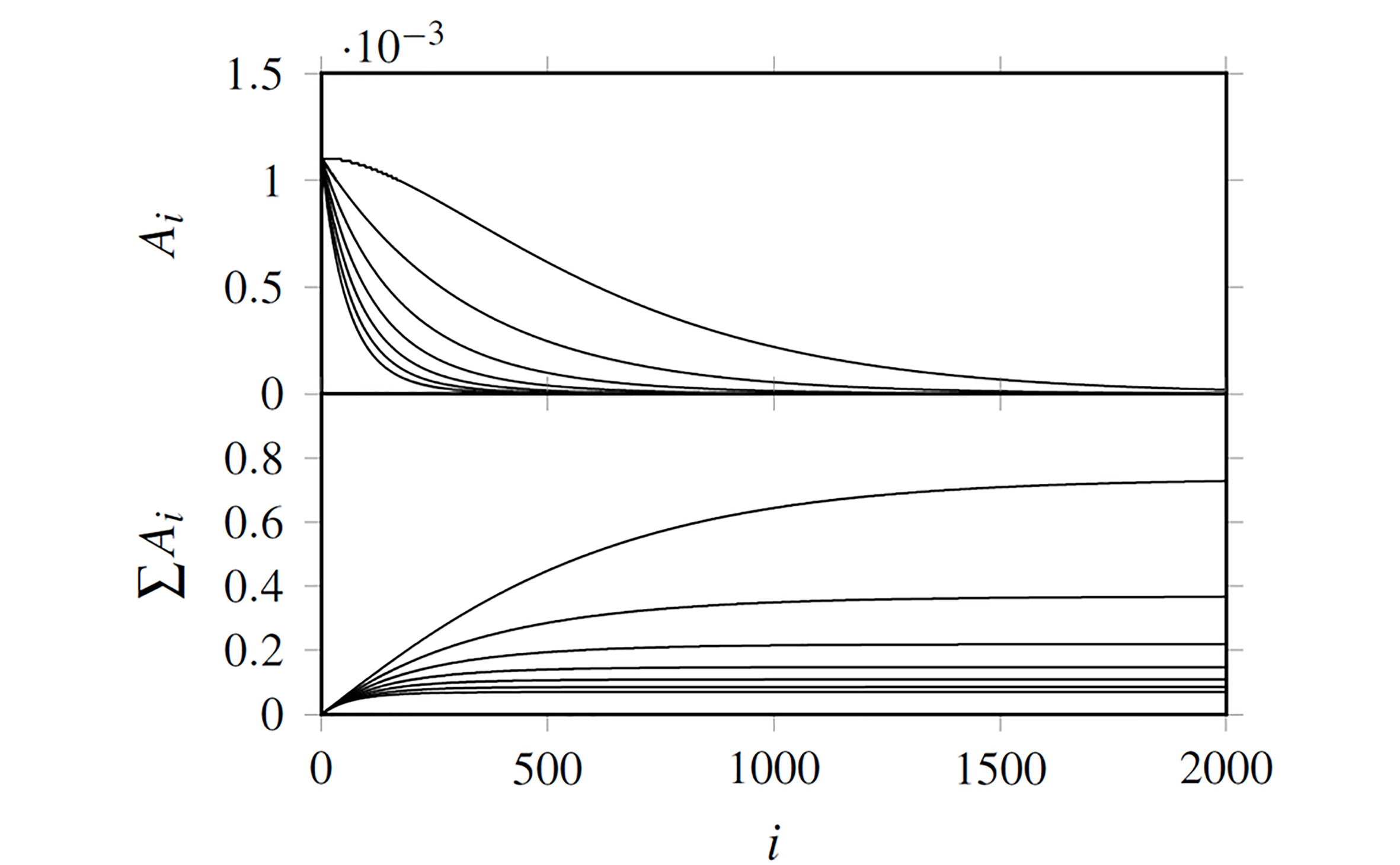
Figure 2 Areas from Simpson 3/8 rule integration (𝐴_𝑖, Eq.(7), upper half) and result 𝑝_𝑚(𝑥)= ∑ⁱ ₁ 𝐴_𝑖 (Eq.(6), lower half) as function of 𝑖. Results are shown for m= −3,−2,…,3 with 𝑥= 1 (own source) 

The calculation is stopped at 𝐴_𝑖∞ and given that all subsequent areas are negligible

Then, dividing by ∑1i∞-1Ai

The index 𝑖_∞ is idenjpgied using the floating point arithmetic’s machine epsilon, which is eps= 2⁻⁵²≈2.220(10⁻¹⁶ for 64 bit double precision variables ²⁵. It is the amount such that numerically

Hence, from the analogy between equations (11) and (12) 𝑖_∞ is the index 𝑖 of the first 𝐴_𝑖 such that

And the calculation is stopped when such condition is reached. Therefore, from Equation 7 the equivalent upper integral limit is 𝑥_∞= χ_3,𝑖∞, where 𝑖_∞ is the last term in the sum.

The use of 𝑖_∞ produced 𝑥_∞ values well below 750, as shown in Figure 3, and allowed to compute the temperature integrals in a reasonable time. For the same 𝑥 (lower limit of temperature integral), 𝑥_∞ decreases with the power 𝑚 because it produces smaller 𝑓(χ) values, and the area sum reaches the point 𝑖_∞ where 𝐴_𝑖∞ becomes insignificant with less terms. On the other hand, higher 𝑥 values produce smaller initial 𝐴_𝑖 values and it is compensated with more terms for the sum ∑1i∞-1Ai in Eq. (13), consequently 𝑥_∞ increases with 𝑥.

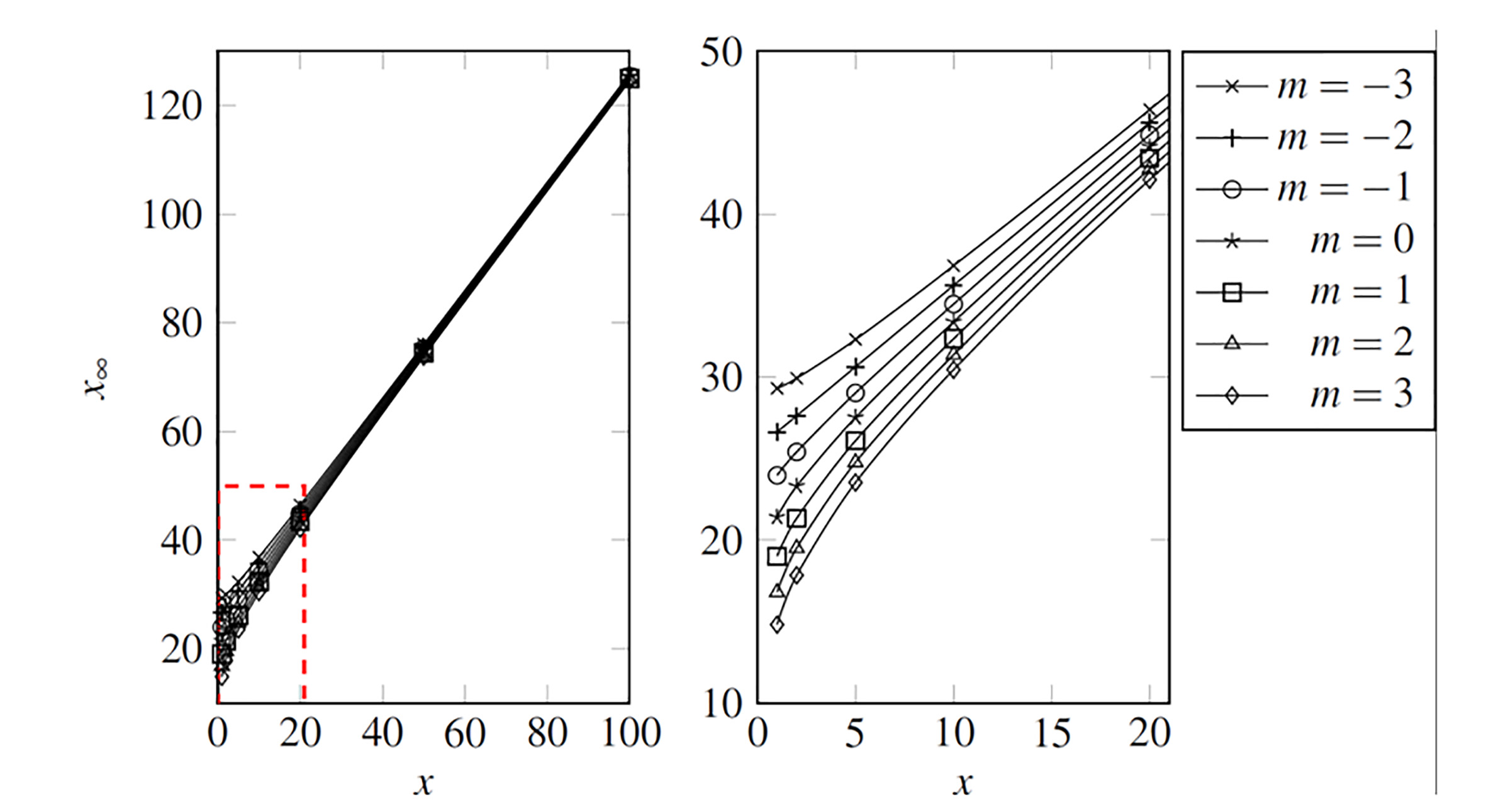
Figure 3 Upper limit, 𝑥_∞ for the integral 𝑝_𝑚, calculated from 𝑖_∞ in Eq. (13). The right plot is a zoom of the area in the red rectangle. Results are shown for different 𝑚 values (own source) 

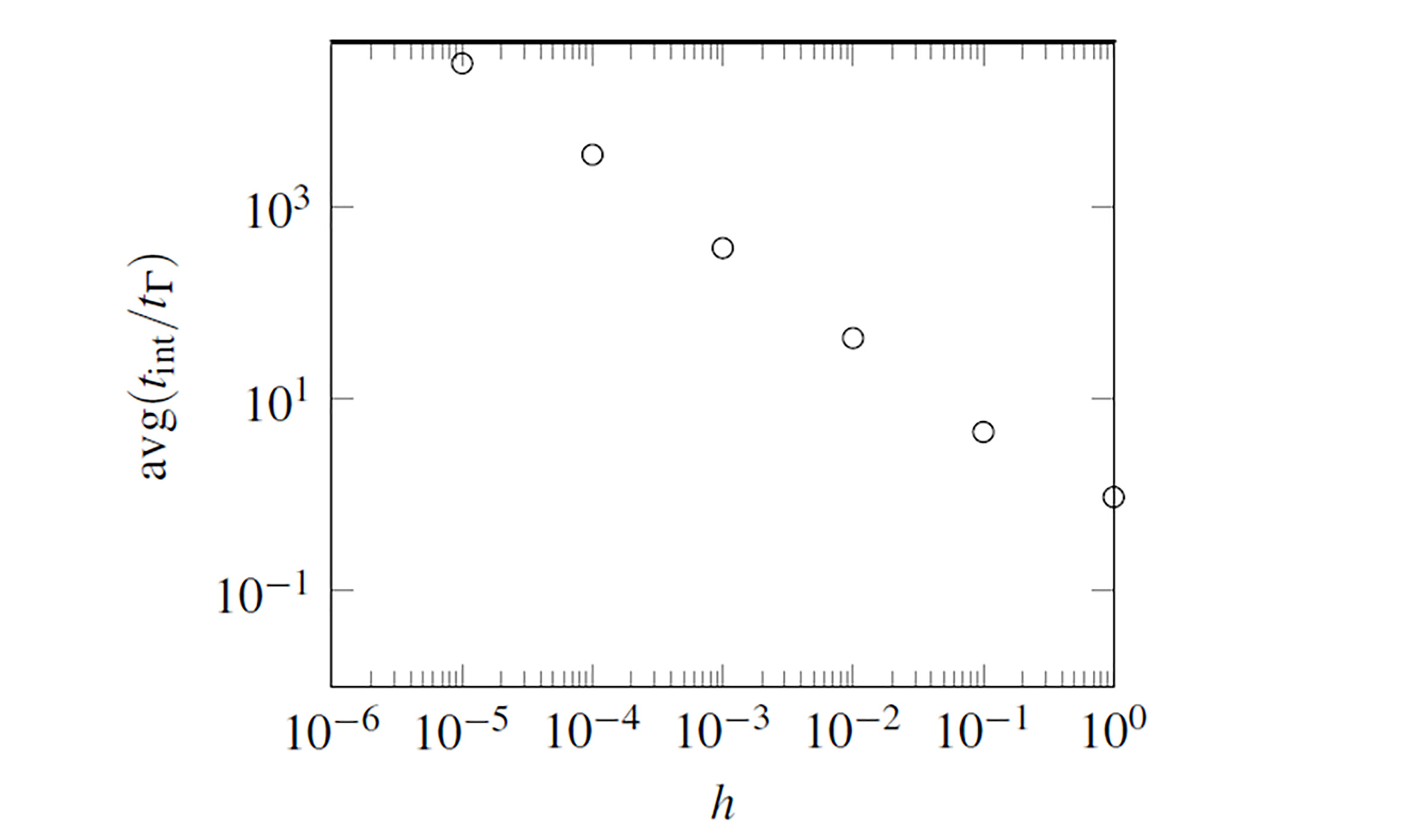
Evaluation of the temperature integral through numerical integration seems less efficient than the use of special functions, but it has not been extensively checked: in the only one comparison found in the literature the execution time of the trapezoidal rule integration is longer than in the Senum-Yang approximation by a factor of 10000 ¹⁹. However, numerical integration can be longer than necessary if the stepsize is too small (the number of evaluations is inversely proportional to ℎ), albeit this minimize the implicit truncation error. In fact it was observed that even results obtained with ℎ≈1 can have an acceptable accuracy. Due to this the effect of stepsize was analyzed comparing execution times from numerical integration and the incomplete gamma function (the representation of 𝑝_𝑚 in terms of Γ is explained in the next section), measured in the same computer, that is, with the same combination of hardware and software, for 10⁻⁵ ≤ ℎ ≤1. The results in Figure 4 show that Simpson 3/8 integration requires more time than the incomplete gamma function, unless stepsize is close to 1.

Figure 4 Averaged quotient of execution times (t, numerical integration)/ (t, incomplete gamma function) (own source)  

4. Calculation based on formulas

Despite the computational raw power available in current computers it is more practical to have a representation of 𝑝(𝑥) as a function than calculating it from numerical integration (in this work with Simpson 3/8 rule) each time it is required. However, the representations of 𝑝(𝑥) found in the literature have limitations. The series (Equation 14)

Where 𝛾= 0.5772156649⋯ is the Euler-Mascheroni constant, is valid for 𝑥< π ^15,26. In the same way the expansion in series of Bernoulli numbers (Equation 15)

Is valid for 𝑥≤2 ^1,27. Multiple integration by parts generates the asymptotic expansion (Equation 16)

But it is reliable only for large 𝑥 values, namely 𝑥>20 ^1,15. The Schlömilch expansion (Equation 17)

Has been used occasionally to produce 𝑝(𝑥) tables, but it is limited and its results may not be precise ^1,15,27,28.

To overcome the limitations of the available 𝑝(𝑥) representations (Eq. 14-17) the values of the temperature integrals were rewritten in terms of the more common special functions: the exponential integrals 𝐸₁ and 𝐸_𝑛; and the incomplete gamma function, Γ. In this way 𝑝(𝑥) becomes in Equation 18 ²⁹

While there are two possible forms for 𝑝_𝑚 (Equation 19):

And (Equation 20)

Which is a consequence of the special case (Equation 21) ⁴

Moreover, the temperature integral 𝑝(𝑥) can also be written in terms of these 𝑝_𝑚 expressions, with 𝑚=0.

Special functions are defined in Equations 22, 23and 24

The exponential integral 𝐸₁ was calculated with the common series expansion (Equation 25) ^30-32

but in this work it was found that for 𝑥>10 it results necessary to use the alternate divergent series form (Equation 26) ³⁰

with 𝑁=15 to obtain complete agreement with values tabulated in the Handbook of Mathematical Functions ³². The incomplete gamma function was calculated with the continued fraction of the Equation 27

using the Lentz algorithm ²¹. Γ(𝑎, 𝑥) was evaluated even with non-integer and negative values of 𝑎, and these results were checked with values from Wolfram’s function site ³³. The numerical evaluation of 𝐸_𝑛(𝑥) is very similar to the procedure for Γ(𝑎,𝑥) because this exponential integral is a special case of the incomplete gamma function (Equation 32) ^21,31,34

with

and

In the general case with 0≤𝑥≤1 (Equation 29)

And the result if 𝑥 ≈>1 comes from the continued fraction in the Equation 30:

As expected 𝑝(𝑥) results from 𝑝_𝑚=0(𝑥), 𝑥⁻¹𝐸₂(𝑥), and Γ(−1,𝑥) coincided, but a further comparison of 𝑝_𝑚(𝑥) against numerical integration is presented in the following section.

5. Comparison

Temperature integral values from 𝐸_1, 𝐸₂, and Γ (see Section 4) were compared against the reference results defining the relative error as follows in the Equation 31:

Where 𝑝_𝑚,intg is the reference value obtained from Simpson 3/8 numerical integration with ℎ= 10⁻⁵.

Results from incomplete gamma function, including 𝑚=0, are summarized as follows:

6. Conclusion

The temperature integral can be computed as 𝑝_𝑚(𝑥) = Γ(−(𝑚 +1),𝑥) for any 𝑚, integer or non-integer and 1≤𝑥≤100. Application of the exponential integral, 𝐸_𝑚+2, is restricted to integer 𝑚 values such that 𝑚≥−2. The incomplete gamma function is preferable to the exponential integral because application of 𝐸₁ to calculate 𝑝(𝑥), although valid, can produce higher relative errors than the other two functions for high 𝑥 values.