


 English (pdf)
 Article in xml format
 Article references
 Send this article by e-mail
 Cited by SciELO
  Cited by Google
  Similars in
SciELO
Similars in
SciELO  Similars in Google
 Permalink
1. Introduction
Research about the Flow-shop Scheduling Problem (FSP) is extensive and the interest on this problem does not abate. A key reason for the continued interest in the FSP is that it represents how many real-world production systems operate; a product requires a sequence of steps performed by different resources with the constraint that each step of the process must be completed for the next to start 1. Researchers have addressed many variations of the FSP considering the diverse settings and characteristics of our industrial world. Some problem versions allow skipping steps 2, others have multiple parallel machines per step 3, and others include due date windows 4.
This paper considers one of the most basic cases of the FSP, called the permutation flowshop problem where all jobs must be processed in the same order in each of the steps, there is a single machine per step, and there is no waiting or setups between jobs and between machines. The key difference with previous work, and the contribution of this article to FSP research, is that the proposed model and analysis considers the case where the resources (the machines) have heterogeneous deterioration based on the job sequence. This research considers two measures of performance: the completion time of the last job on the schedule (e.g., the makespan) and the average tardiness. These two are among the most commonly addressed measures in the FSP literature 5-7.
Research in the flowshop problem with deterioration has been previously addressed by multiple authors. Research that addresses the minimization of the makespan include Kononov and Gawiejnowicz 8, Wang and Xia 9, Wang et al. 10, Lee et al. 11, Lee et al. 12, Wang et al. 13, Wang and Wang 14 and Sun et. al 15. With the exception of 13, the models addressed by these authors considers the processing time as a linear function which is dependent on its starting time: the time to process a job j in machine 𝑘 is assumed to be 𝑎 j,𝑘 + λ j,𝑘 where 𝑎 j,𝑘 is the basic processing time of job j in machine 𝑘, λ is the deterioration rate, and 𝑡 j,𝑘 is the start time of job j in machine 𝑘. In Wang et al. 13 the position of the job is relevant, noting their model includes both deterioration and learning. Under this model the time to process a job j in machine 𝑘 is assumed to be 𝛼 j,𝑘 𝑡𝑟𝑏 where 𝛼 j,𝑘 is the deterioration rate of job j on machine 𝑘, 𝑡 is the start time of job j on machine 𝑘, and 𝑟 is the position of job j on the schedule, and 𝑏 is the learning index (𝑏 ≤ 0).
Research that addresses the minimization of the total tardiness for the flowshop problem with deterioration has not received much attention, with Bank et al 16 and Lee et al. 17 being the only two articles on the subject. As in most of the pervious papers, the deterioration of the jobs is based on a linear function of their starting times. Research in the related measure of maximum tardiness by Sanchez-Herrera et al. 18 considers position-based deterioration.
Therefore, previous research typically considers the situation where the jobs deteriorate depending on the time at which they start being processed or based on their position in the sequence. This view of the system fails to consider environments where the machines (or worker) are the elements that are wearing down/deteriorating, and each job may have a different effect on the condition of the machine. Therefore, a job’s processing time would not depend on the start time, or the number of jobs previously processed (position), but rather in the condition of the machine, where the condition of the machine does not depend on the time or just the number of jobs, but rather on the specific set of jobs processed. An approach to model deterioration in this manner was proposed by Ruiz-Torres et al. 19 and has been used in several follow up work including Santos and Arroyo 20, De Araújo et al. 21, Perez et al.22 and Ding et al.23.
Furthermore, this approach to modeling deterioration is an element of a software developed for the optimization of logistics during well drilling 24. As in the case of drilling, there are multiple real-world settings where the equipment (machines) deteriorates based on the particular sequence, for example processes associated with metal cutting and shredding where equipment performance decreases as it processes the materials. The cutting tools’ characteristics in terms of sharpness and hardness deteriorates due to the heat and pressures of the involved processes, and as this occurs, the time required to process a job in order to meet the required specifications will increase in comparison with the original plan. However, the wear/deterioration effect on the machine is not the same for all jobs being processed.
For instance, material that is softer will have a smaller effect than material that is harder. For example, at time 𝑡= 35 a set of easy jobs would have been completed and as a result the machine would be performing at 90%. In this case the time to process job j would be 5 hours to complete given the machine status. On the other hand, if at time 𝑡 = 35 a set of hard jobs would have been completed and, therefore, the machine would be performing at 75%. In this case, the time to process job j would be 6 hours. Another simple illustrative example relates to a person doing exercises following a multi-step routine. This person can either start the routine by running 2 kilometers or walking 1.5 kilometers (and we assume this person can complete any of them in 12 minutes at the start of the routine - when “fresh”). For most people, the level of deterioration (tiredness) for position 2 (second exercise of the routine) or conversely at time = 12 minutes would be very different depending on the decision of what exercise to do first (run or walk), and thus performing the next exercise may take different amounts of time in each case.
Given the time to process jobs increases as the machines degrades, a simple option is to run the softer jobs first. However, this simple approach is only true if all jobs have the same processing times 19. It is worthwhile noting that the proposed model also has direct application to the scheduling of people. The sequence of jobs performed by an operator can have diverse effects on the level of mental/physical tiredness of that person, therefore a type of deterioration. This is probably the reason why many people like to do the easy tasks first.
This research contributes to the body of knowledge in production and engineering as it takes on a different view of the system concerning deterioration in flowshop scheduling, where the machines deteriorate based on the set of jobs previously processed by the resource. Furthermore, this research is relevant as it expands on the study of the effect that deterioration has on the tardiness criteria, which is relevant in customer service and therefore competitiveness. This paper is organized as follows; Section 2 provides the methodology including the problem description and heuristics proposed to generate schedules, Section 3 presents computational experiments and results, while Section 4 provides conclusions and directions for future work.
2. Methodology
2.1. Problem description
Consider a set 𝑁= {1, … j, … 𝑛} of 𝑛 independent jobs to be processed on a flowshop with two machines. All jobs flow in the same sequence (permutation flowshop), from machine 1 to machine 2. All jobs are available at time 0 (static case) and cannot be preempted or divided. Each machine can process only one job at a time. At time 0 (the start of the schedule) both machines are at their baseline state (e.g., 0% wear = 100% performance). Let 𝑝 j,𝑘 be the baseline processing time of job j on machine 𝑘; 𝑤 j,𝑘 be the wear/deteriorating effect of job j on machine 𝑘 with 0 ≤ 𝑤 j,𝑘 ≤ 1, and let 𝑑 j be the due date of job j.
Let X be the ordered set of jobs and 𝑥 [ ℎ ] be the job assigned to position ℎ. Let 𝑞ℎ,𝑘 be the performance level for the job in position ℎ of machine 𝑘. For 𝑘= 1,2 the value of 𝑞ℎ,𝑘 is defined by (1 − 𝑤𝑥[ ℎ−1], 𝑘) ( 𝑞ℎ-1𝑘 when > 1, and 𝑞ℎ,𝑘 = 1 when ℎ = 1 (as mentioned earlier, the model assumes the machines are at their “best” operating level at the start of the schedule). Let 𝑝′𝑥[ℎ],𝑘 be the actual processing time of job 𝑥 [ ℎ ] in machine 𝑘, and 𝑝′𝑥[ℎ],𝑘 = 𝑝𝑥[ℎ],𝑘⁄𝑞ℎ,𝑘. This function to define resource deterioration was first used in 19 and used in follow up research as mentioned in the Introduction section 20-23.
The completion time of a job j in machine 𝑘 is 𝑐 j,𝑘 and the tardiness of a job is 𝑡 j = max [0, 𝑐j,2 − 𝑑j] . The measures under analysis are the makespan: 𝑐max = max j(𝑁 𝑐 j,2 and the average tardiness: 𝑡𝑎𝑣𝑒 = ∑ j(𝑁 𝑡 j ⁄𝑛.
A simple example is presented next to illustrate the problem. There are 𝑛 = 6 jobs with processing times, wear/deterioration, and due dates parameters as in Table 1. We first consider the makespan measure of performance and use Johnson’s algorithm 25 to determine a schedule given it provides the optimal solution in the basic case with no wear/deterioration. Note that Johnson Algorithm (JA) iteratively selects the job with the smallest processing time in any of the machines and assigns them to the sequence: if the process time is in machine 1, the job is placed in the “front” of the schedule, and if it’s on the second machine, its placed on the “back” of the schedule, working towards the center of the sequence until all jobs are assigned (a formal description is provided in section 2.2.2).
Table 1 Job information
| j | 𝑝 j,1 | 𝑝 j,2 | 𝑤 j,1 (%) | 𝑤 j,2 (%) | 𝑑 j |
|---|---|---|---|---|---|
| 1 | 34 | 51 | 2 | 5 | 100 |
| 2 | 80 | 30 | 6 | 6 | 145 |
| 3 | 25 | 60 | 1 | 7 | 210 |
| 4 | 48 | 45 | 9 | 2 | 260 |
| 5 | 60 | 18 | 5 | 1 | 280 |
| 6 | 20 | 50 | 4 | 9 | 350 |
Therefore for this example, job 5 is selected first and placed at the “back” of the schedule, then job 6 is selected and placed at the “front”, then job 3 is selected and placed at the front (but after 6), then job 2 is placed at the “back”, but ahead of job 5, next is job 1 which is placed at the front (but after 3), and finally job 4 stays in the middle remaining position for the sequence: 6-3-1-4-2-5.
The top diagram of Figure 1, schedule s1, presents the JA based schedule with no machine wear/deterioration (in other words 𝑤 j,1 = 𝑤 j,2 = 0 ⩝ ( 𝑁). Schedule s1 includes the completion time of each job on each of the two machines. This schedule has a makespan of 285, which as mentioned is optimal when no machine wear/deterioration is considered. Schedule s2 of Figure 1 presents the same sequence of jobs but including machine deterioration. The diagram includes the completion time of each job on each machine as well as the machine performance level at the end of that job (position assigned to that job).
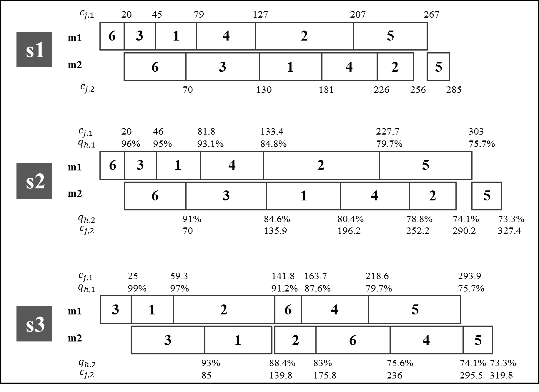
Figure 1 Three schedules: JA not considering wear/deterioration (s1), JA considering wear/deterioration (s2), optimal makespan schedule considering wear/deterioration (s3)
Next, it is described how the machine’s performance level and the actual job’s processing times are determined when machine wear/deterioration is considered. The performance level of machine 1 is at 100% in position 1 (ℎ = 1, 𝑞1,1 = 1), the position assigned to job 6. The actual process time of job 6 is 20 (𝑝′6,1 = 𝑝6,1⁄𝑞1,1 = 20⁄1 = 20). Given 𝑤6,1 = 4%, the machine performance level at the end of job 6 (therefore for position ℎ = 2) is 96% (𝑞2,1 = (1− 𝑤6,1) ⨯ 𝑞1,1 = 0.96 ⨯ 1 = 0.96). The actual process time for job 3 (the job assigned to position 2) is 26 (𝑝′3,1 = 𝑝3,1⁄𝑞2,1 = 25⁄0.96 = 26). Given 𝑤3,1 = 1%, the performance level of machine 1 after job 3 (therefore for position ℎ = 3) is 95.04% (𝑞3,1 = (1− 𝑤3,1) ⨯ 𝑞2,1 = 0.99 ⨯ 0.96 = 0.9504). The actual process time for job 1 (the job assigned to position 3) is 35.8 (𝑝′1,1 = 𝑝1,1⁄𝑞3,1 = 34⁄0.9504 = 35.08). The same calculations are repeated for the remaining positions and for machine 2 (considering the availability for the job in the second machine). It is noted that the performance level at the end of the schedule will be the same value for all possible sequences as it is the effect of processing all jobs in the machine (total wear/deterioration). The makespan of this schedule is 327.4, a difference of almost 15% versus the case when machine deterioration is not considered (Schedule 1 of Figure 1). Schedule s3 in Figure 1 presents a third schedule considering machine wear/deterioration with a makespan of 319.8. This sequence was obtained by a full enumeration search (in other words, all possible schedules were generated) and it results in the lowest makespan for the example problem. It is evident with this example that the schedules generated by JA are not optimal for the proposed problem.
Figure 2 presents the schedules generated when ordering jobs according to the Earliest Due Date rule (EDD). Schedule s4 illustrates the schedule when machine wear/deterioration is not considered and the bottom schedule when it is considered. The jobs in grey are late. The additional row of information below the schedule is the tardiness for each job (𝑡 j ). When machine wear/deterioration is not considered, all the jobs are on time, therefore an average tardiness of 0 (Schedule s4). As it can be noted in schedule s5 of Figure 2, when machine wear/deterioration is considered, five jobs are tardy with an average tardiness of 5.18. From the previous discussion, it should be clear that ignoring machine wear/deterioration is very important as it could lead to incorrect/poor decisions in work planning.
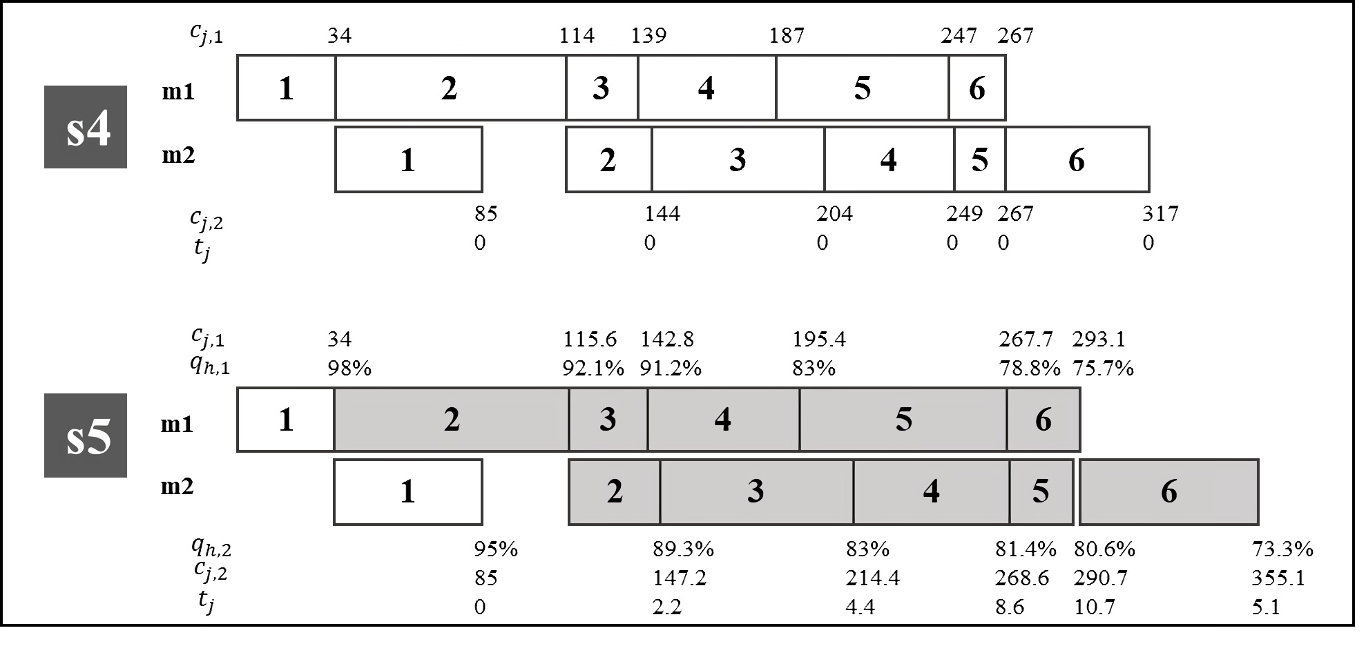
Figure 2 Two schedules ordered by due date, one not considering wear/deterioration (s4) and another considering wear/deterioration (s5)
2.2 Heuristics
This section describes basic algorithms used to generate job sequences and improve on the resulting measures of performance. The algorithms used to generate job sequences are based on list ordering and on Johnson’s algorithm. The improvement methods are based on job exchange strategies.
2.2.1 Ordering using one job characteristic
The job sequence is based on a single characteristic for each job. Eight characteristics are analyzed, where in all cases the list is in non-decreasing order of the characteristic.
EDD: due date (𝑑 j ).
Slack: slack time based on the baseline process times (𝑠 j = 𝑑 j − 𝑝 j , 1− 𝑝 j , 2).
w 1: wear/deterioration effect on the first machine (𝑤 j,1 ).
w 2: wear/deterioration effect on the second machine (𝑤 j,2 ).
p 1: baseline process time on the first machine (𝑝 j , 1).
p 2: baseline process time on the second machine (𝑝 j , 2).
p_w 1: ratio of baseline process time over the performance level effect on the first machin (𝑝 j , 1⁄(1 − 𝑤 j,1 ))
p_w 2: ratio of the baseline process time over the performance level on the second machine (𝑝 j , 2⁄(1 − 𝑤 j,2 )).
2.2.2 Ordering using two job characteristics
The job sequence is created by using information from both machines. Three rules are analyzed that use the wear/deterioration effects, the baseline process times, and the ratio of process time to performance level. The first rule is in principle similar to Johnson’s but attempts to assign the jobs with lower wear/deterioration effect in the first machine at the front of the sequence, and the jobs with higher wear/deterioration jobs in the second machine at the “back” of the sequence. The second and third algorithms are Johnson’s and a modified version that uses the ratio characteristic, respectively.
Wear effect algorithm (WA)
Step 1. Let
Step 2. Let
Step 3. Let
Step 4. If
Step 5. Let
Step 6. If
Johnson’s algorithm (JA)
Step 1. Let
Step 2. Let
Step 3. If
Step 4. Let
Step 5. If
Modified Johnson’s algorithm (MA)
Step 1. Let
Step 2. Let
Step 3. If
Step 4. Let
Step 5. If
2.2.3 Improvement methods
These improvement methods exchange jobs to reduce the measure of performance under consideration. Let 𝑣 be the current value of the measure of performance of interest (makespan or average tardiness) for a schedule with job sequence 𝑋. As in Wang et al.13 the First Improvement (FI) method accepts the first exchange that results in an improvement in v, while in the Best Improvement (BI) method, all exchanges are considered, and the best exchange is accepted. Both versions end when no further improvements are found.
First improvement (FI)
Step 1. Let 𝑦 = 1 and 𝑧 = 2.
Step 2. Let job 𝑎 = j [ 𝑦] and job 𝑏 = j [𝑧 ].
Step 3. Exchange the positions of jobs 𝑎 and 𝑏 and let 𝑣' be the measure of performance of this sequence.
Step 4. If 𝑣' < 𝑣 then let 𝑣 = 𝑣' and return to Step 1.
Step 5. Exchange the positions of jobs 𝑎 and 𝑏.
Step 6. If 𝑧 < 𝑛 let 𝑧 = 𝑧 + 1 and return to Step 2.
Step 7. If 𝑦 < 𝑛 - 1 then 𝑦 = 𝑦 + 1 and 𝑧 = 𝑦 + 2 and return to Step 2.
Best improvement (BI)
Step 1. Let 𝑦 = 1, 𝑧 = 2, and 𝑣 best = 𝑣.
Step 2. Let job 𝑎 = j 𝑥 [ 𝑦] and job 𝑏 = j 𝑥[𝑧 ].
Step 3. Exchange the positions of jobs 𝑎 and 𝑏 and let 𝑣' be the measure of performance of this sequence.
Step 4. If 𝑣' < ?? best , then let 𝑣 best = 𝑣', 𝑦 best = 𝑦, 𝑧 best = 𝑧.
Step 5. Exchange the positions of jobs 𝑎 and 𝑏.
Step 6. If 𝑧 < ?? let 𝑧 = 𝑧 + 1 and return to Step 2.
Step 7. If 𝑦 < 𝑛 - 1 then 𝑦 = 𝑦 + 1 and 𝑧 = 𝑦 + 2 and return to Step 2.
Step 8. If 𝑣 best < 𝑣 then let job 𝑎 = j 𝑥 [𝑦best] and job 𝑏 = j 𝑥[𝑧best] , exchange the positions of jobs 𝑎 and 𝑏, let 𝑣 be the measure of performance of this sequence and return to Step 1.
2.2.4 Overall set of Heuristics
A total of 11 heuristic approaches are proposed to generate an initial schedule (8 presented in section 2.2.1 and 3 presented in section 2.2.2), while two improvement heuristics are described in section 2.2.3. Therefore, a total of 22 combination approaches (initial sequence followed by an improvement heuristic) can be generated. For the makespan criteria the initial sequence based on due date and slack are not relevant, therefore 18 applicable heuristic combinations remain.
3. Results y discussion
Two sets of experiments are conducted to evaluate the performance of the heuristic for the two criteria under consideration. The first set of experiments evaluate the heuristic performance versus the optimal solution for small sized problems (optimal benchmark experiments), while the second set of experiments evaluate relative heuristic performance for larger sized problems (relative benchmark experiments). To find the optimal solution for the first set of experiment, a full enumeration search is conducted where all the possible job sequences are examined, and the schedules are generated. All experiments were conducted on a personal computer with the following characteristics: 12GB RAM, 2.9GHz CPU, Windows 10 OS.
3.1 Experimental Framework
Four experimental variables are considered: the number of jobs, the range of process times, the range of wear/deteriorations, and the congestion ratio. For the optimal benchmark experiments 𝑛 is considered at two levels: 𝑛 = 6, 8 while for the relative benchmark experiments 𝑛 is considered at three levels: 𝑛 = 10, 15, 20. For the relative evaluation experiments, the value of 𝑛 = 20 is selected as the largest level as higher values of 𝑛 are deemed unpractical. At larger values of 𝑛, the machine performance levels would be excessively low, and in such cases including maintenance events would be “required” (an area of future research). It is also noted that a problem with 𝑛 = 20 has 20! possible sequences, which is already quite a large number of combinations.
The processing times for the jobs are randomly generated using a uniform distribution with range 𝑝 min,𝑘 to 𝑝 max,𝑘 , and the wear/deteriorations are randomly generated using a uniform distribution with range 𝑤 min,𝑘 to 𝑤 man,𝑘 . These two experimental factors are considered at four levels as described in Table 2. For the processing times, and based on the expected values, the first level represents the case where both machines have high variability and have an equal average load; the second level represents the case where both machines have less variability and the same average load; the third level represents the case where there is more variability in the first machine and the second machine has a higher processing load, and the fourth level represents the case where the first machine has a higher average load and the second machine has more variability.
Table 2 Experimental levels for variables 𝑝range and 𝑤range.
| 𝑝range level name | 𝑝 min,1 , 𝑝 max,1 | 𝑝 min,2 , 𝑝 max,2 |
|---|---|---|
| hv_hv | 1, 100 | 1, 100 |
| hl_hl | 50, 100 | 50, 100 |
| hv_hl | 1, 100 | 50, 100 |
| hl_hv | 50,100 | 1,100 |
| 𝑤range level name | 𝑤 min,1 , 𝑤 max,1 (%) | 𝑤 min,2 , 𝑤 max,2 (%) |
| lw_lw | 0, 5 | 0, 5 |
| hw_hw | 5, 10 | 5, 10 |
| lw_hw | 0, 5 | 5, 10 |
| hw_lw | 5,10 | 0, 5 |
For the wear/deterioration factor and also based on expected values, the first level represents the case where the jobs have a low effect in both machines, the second level represents the case where the jobs have a high wear/deterioration effect in both machines, the third level represents the case where the jobs deteriorate the first machine significantly less than the second machine, and the fourth level represents the case where the jobs deteriorate the first machine significantly more than the second machine.
The due date for a job j is randomly generated using a uniform distribution with range 𝑑 min to 𝑑 max . The value of 𝑑 min = 𝑝 j,1 + 𝑝 j,2 , while 𝑑 max = (∑𝑔∊𝑁 𝑝𝑔,1 + 𝑝𝑔,2)⁄θ, where θ is called the due date tightness ratio. The experimental factor θ is considered at three levels 1, 1.5 and 2, and as it increases the due dates decrease while the average tardiness is expected to increase. One randomly selected job of every instance is assigned a 𝑑 j = 0, thus for all instances 𝑡𝑎𝑣𝑒 ≥ 0.
For the optimal benchmark experiment set there are 2 X 4 X 4 experimental combinations when the makespan is considered (θ is not relevant), and 2 X 4 X 4 X 3 for the average tardiness measure. For the relative benchmark experiment set there are 3 X 4 X 4 experimental combinations for the makespan measure, and 3 X 4 X 4 X 3 for the average tardiness measure. For each experimental combination 10 replications are generated. For the optimal benchmark problems, all possible sequences are generated to find the optimal sequence. For the relative benchmark experiments, the best solution found by the heuristics is considered the “optimal”, although the true optimal is unknown.
3.2 Makespan Results
Table 3 presents for each experimental level the mean makespan and the percentage of times that at least one of the heuristics found the optimal solution. At least one of the heuristics found the optimal solution in 98.1% (314 out of 320) of the instances and under the hv_hv and lw_lw levels of 𝑝range and 𝑤range respectively, the optimal makespan was found in 100% of those instances. As a set, the heuristics provide a very good approximation to the optimal within the analyzed structure, although as can be noted, as 𝑛 increases the % of optimal solutions obtained decreases, and the condition of 𝑝range = ℎ𝑣_ℎ𝑙 and 𝑤range ℎ𝑤_ℎ𝑙 results in a lower percentage of optimal solutions found.
Table 3 Mean makespan and percentage of optimal solutions found by at least one heuristic
| 𝑐 max | % optimal | ||
|---|---|---|---|
| 𝑛 | 6 | 514.0 | 98.8 |
| 8 | 700.3 | 97.5 | |
| 𝑝range | hv_hv | 460.1 | 100.0 |
| hl_hl | 719.6 | 98.8 | |
| hv_hl | 620.8 | 96.3 | |
| hl_hv | 628.4 | 97.5 | |
| 𝑤range | lw_lw | 557.2 | 100.0 |
| hw_hw | 650.2 | 98.8 | |
| lw_hw | 606.7 | 98.8 | |
| hw_lw | 614.7 | 95.0 | |
| Overall | 607.2 | 98.1 |
The discussion of the results focuses on the best performing subset of heuristics in order to emphasize the more relevant solution approaches. Table 4 presents the percentage of times each heuristic generated the optimal solution. The values in bold indicate the highest percentage for that experimental level. The best overall performer is MA-BI which found 83.8% of the optimal solutions, followed by JA-BI which generated 83.4% optimal solutions. These two heuristics dominated in five experimental levels; however, they do not dominate across all the experiments; five of the heuristics dominate in at least one level. A notable heuristic is w1-BI which outperforms all others at two experimental levels with a relatively high success rate, finding 88.8% and 90% of the optimal values for 𝑝range = ℎ𝑙_ℎ𝑣 and 𝑤range 𝑙𝑤_ℎ𝑤 respectively. It is noted that the BI improvement approach on average outperforms the FI approach.
Table 4 Percentage of the optimal makespan solutions generated by the heuristic
| Heuristic | JA | JA | MA | MA | p1 | p1 | w1 | w1 | |
|---|---|---|---|---|---|---|---|---|---|
| FI | BI | FI | BI | FI | BI | FI | BI | ||
| 𝑛 | 6 | 83.1 | 83.8 | 82.5 | 84.4 | 80.0 | 85.6 | 78.1 | 85.0 |
| 8 | 75.6 | 83.1 | 76.3 | 83.1 | 76.9 | 80.6 | 73.1 | 75.6 | |
| 𝑝range | hv_hv | 80.0 | 86.3 | 80.0 | 86.3 | 73.8 | 86.3 | 72.5 | 78.8 |
| hl_hl | 68.8 | 71.3 | 67.5 | 73.8 | 72.5 | 70.0 | 68.8 | 72.5 | |
| hv_hl | 87.5 | 88.8 | 88.8 | 87.5 | 86.3 | 88.8 | 81.3 | 81.3 | |
| hl_hv | 81.3 | 87.5 | 81.3 | 87.5 | 81.3 | 87.5 | 80.0 | 88.8 | |
| 𝑤range | lw_lw | 77.5 | 82.5 | 77.5 | 82.5 | 77.5 | 83.8 | 75.0 | 81.3 |
| hw_hw | 75.0 | 83.8 | 76.3 | 82.5 | 73.8 | 82.5 | 77.5 | 77.5 | |
| lw_hw | 85.0 | 85.0 | 85.0 | 85.0 | 86.3 | 86.3 | 77.5 | 90.0 | |
| hw_lw | 80.0 | 82.5 | 78.8 | 85.0 | 76.3 | 80.0 | 72.5 | 72.5 | |
| Overall | 79.4 | 83.4 | 79.4 | 83.8 | 78.4 | 83.1 | 75.6 | 80.3 |
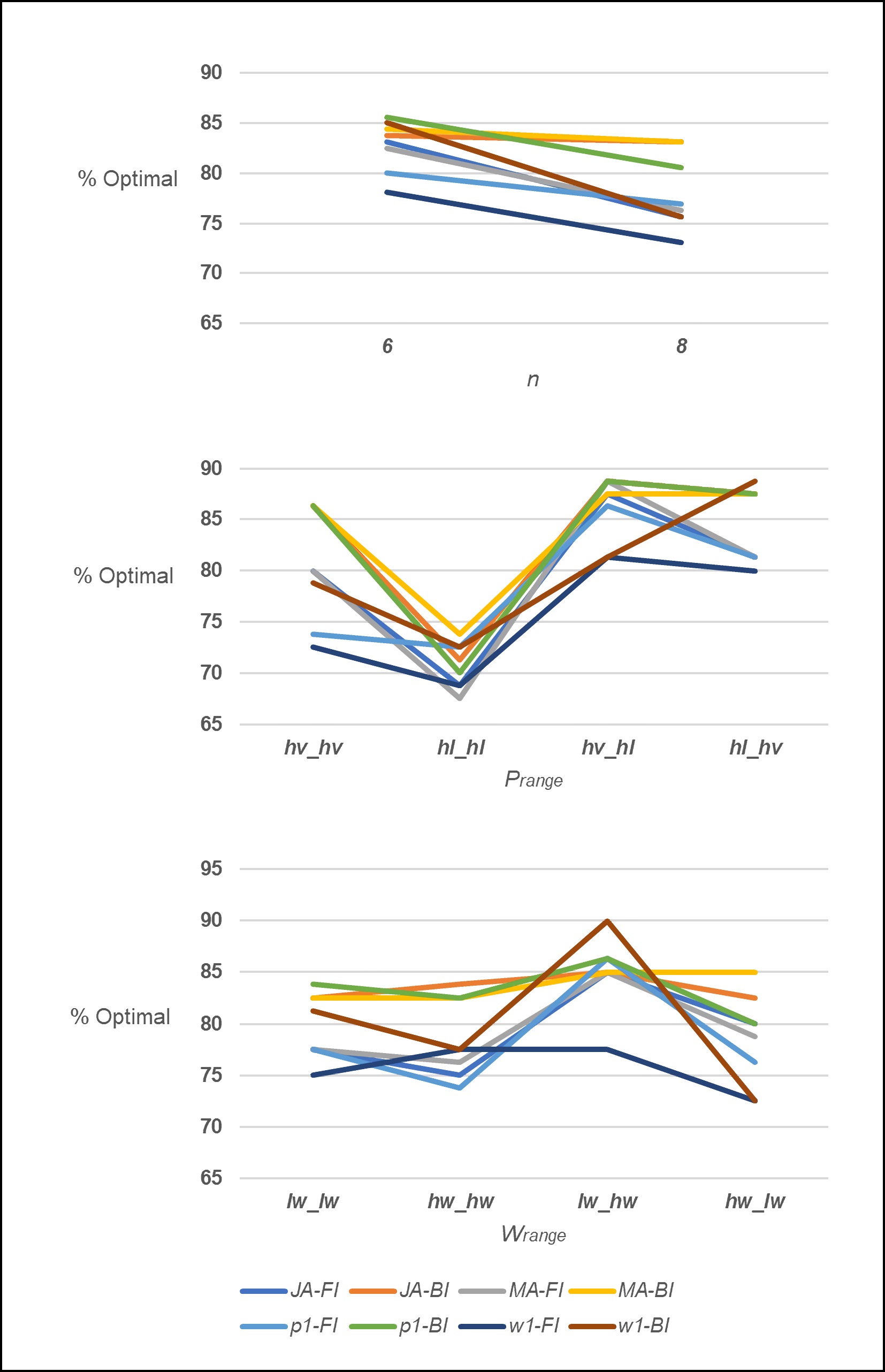
Figure 3 illustrates the results per experimental factor. For the overall set of heuristics, the average number of optimal solutions decreased slightly as 𝑛 increased, with heuristics JA-BI and MA-BI being the exception, maintaining a similar performance level for both values of 𝑛. Heuristic performance changed notably at the different levels of the 𝑝range factor, where at ℎ𝑣_ℎ𝑙 and ℎ𝑙_ℎ𝑣 all heuristics perform relatively well (80-90% of the optimal solutions), at ℎ𝑣_ℎ𝑣 two heuristics perform well (85%+) and the rest have average performances ( 80%, and at ℎ𝑙_ℎ𝑙 where all the heuristic has lower performance levels (( 75%). It is observed that heuristic MA-BI performs well across all levels of 𝑝range in particular for the ℎ𝑙_ℎ𝑙 condition where the process times on both machines is higher. Factor 𝑤range also has an effect on overall performance and heuristic dominance, although heuristics p1-BI, MA-BI, and JA-BI have relatively good performance across all levels. The figure also illustrates how experimental parameters have notable effects on the performance of individual heuristics; for example, heuristic w1-BI performs in the “middle of the pack” for levels 𝑙𝑤_ℎ𝑤 and ℎ𝑤_ℎ𝑤, outperforms all others at 𝑙𝑤_ℎ𝑤, and is the worst performer at ℎ𝑤_𝑙𝑤.
The size of the error when the heuristic does not find the optimal solution is analyzed as a second assessment of overall heuristic performance. Table 5 provides the mean and maximum error versus the optimal for those instances where the heuristic did not find the optimal (𝑒𝑟𝑟𝑜𝑟% = (1 - 𝑐 max [heuristic ]⁄ 𝑐 max [optimal ])⨯100). Heuristics MA-BI and JA-BI are the best performers; for 16.2% of the total instances that MA-BI does not find the optimal solution, the mean error is 0.45% and the worst error is 2.14%. For the 16.6% of the total instances that JA-BI does not generate the optimal solution, the mean error is 0.46% and the worst error is 1.73%. Therefore, even in the cases where the optimal solution is not found, the error is on average less than 0.5%.
Table 5 Mean and maximum error% for instances versus the optimal.
| Heuristic | JA | JA | MA | MA | p1 | p1 | w1 | w1 |
|---|---|---|---|---|---|---|---|---|
| FI | BI | FI | BI | FI | BI | FI | BI | |
| Mean | 0.50 | 0.46 | 0.53 | 0.45 | 1.04 | 0.59 | 0.87 | 1.02 |
| Max. | 2.93 | 1.73 | 3.23 | 2.14 | 12.30 | 4.21 | 6.60 | 7.39 |
Table 6 presents the percentage of instances per experimental level where a heuristic generated the best makespan solution for the relative benchmark experiments. As in the optimal benchmark experiments, the best overall performer is MA-BI which found 63.1% of the best solutions.
Table 6 Percentage of the “best” makespan solutions generated by a heuristic
| Heuristic | JA | JA | MA | MA | p1 | p1 | w1 | w1 | |
|---|---|---|---|---|---|---|---|---|---|
| FI | BI | FI | BI | FI | BI | FI | BI | ||
| 𝑛 | 10 | 65.6 | 74.4 | 65.6 | 74.4 | 70.6 | 72.5 | 71.9 | 66.9 |
| 15 | 61.9 | 59.4 | 61.3 | 60.6 | 58.1 | 59.4 | 59.4 | 60.0 | |
| 20 | 55.6 | 54.4 | 56.3 | 54.4 | 55.0 | 55.6 | 57.5 | 52.5 | |
| 𝑝range | hv_hv | 51.7 | 48.3 | 51.7 | 48.3 | 51.7 | 46.7 | 53.3 | 44.2 |
| hl_hl | 54.2 | 55.8 | 55.8 | 57.5 | 57.5 | 55.8 | 59.2 | 53.3 | |
| hv_hl | 69.2 | 68.3 | 67.5 | 68.3 | 67.5 | 67.5 | 70.0 | 68.3 | |
| hl_hv | 69.2 | 78.3 | 69.2 | 78.3 | 68.3 | 80.0 | 69.2 | 73.3 | |
| 𝑤range | lw_lw | 55.0 | 58.3 | 55.8 | 60.0 | 55.0 | 57.5 | 54.2 | 49.2 |
| hw_hw | 53.3 | 54.2 | 55.0 | 54.2 | 55.8 | 54.2 | 61.7 | 52.5 | |
| lw_hw | 73.3 | 70.0 | 73.3 | 70.0 | 74.2 | 71.7 | 70.8 | 68.3 | |
| hw_lw | 62.5 | 68.3 | 60.0 | 68.3 | 60.0 | 66.7 | 65.0 | 69.2 | |
| Overall | 61.0 | 62.7 | 61.0 | 63.1 | 61.3 | 62.5 | 62.9 | 59.8 |
However, in this set of experiments heuristic w1-FI is the runner up performer, finding the best solution in 62.9% of the problems and dominating in five of the experimental levels. Six of the heuristics outperform the others in at least one experimental level, with w1-FI being the heuristic that outperforms the others in the most cases. As in the optimal benchmark experiment, none of the heuristic outperforms the others across all experimental levels and unlike the optimal benchmark experiments, the FI improvement heuristic outperforms the BI approach on some conditions.
The results by experimental factor for the percent of “best” solutions found are shown in Figure 4. The results are relatively similar to those obtained for the optimal solution, for example, as 𝑛 increased, heuristic performance decreased. Relative heuristic performance also changed at the different levels of 𝑛, where at 𝑛 = 10, heuristic MA-BI outperforms the rest, while at 𝑛 = 20, heuristc w1-F1 is the best performer. The 𝑝range experimental factor had a significant effect on the overall performance: poor at hv_hv and hl_hl and good at hv_hl and hl_hv. At the hv_hv and hl_hv levels, there was a noticeable differentiation in relative performance; for example, at hv_hv, heuristic w1-FI outperformed all others and heuristic p1-BI performed relatively poorly, while at hl_hv, their relative performance “flips”, as p1-BI outperforms all others and w1-FI is one of the worst performers.
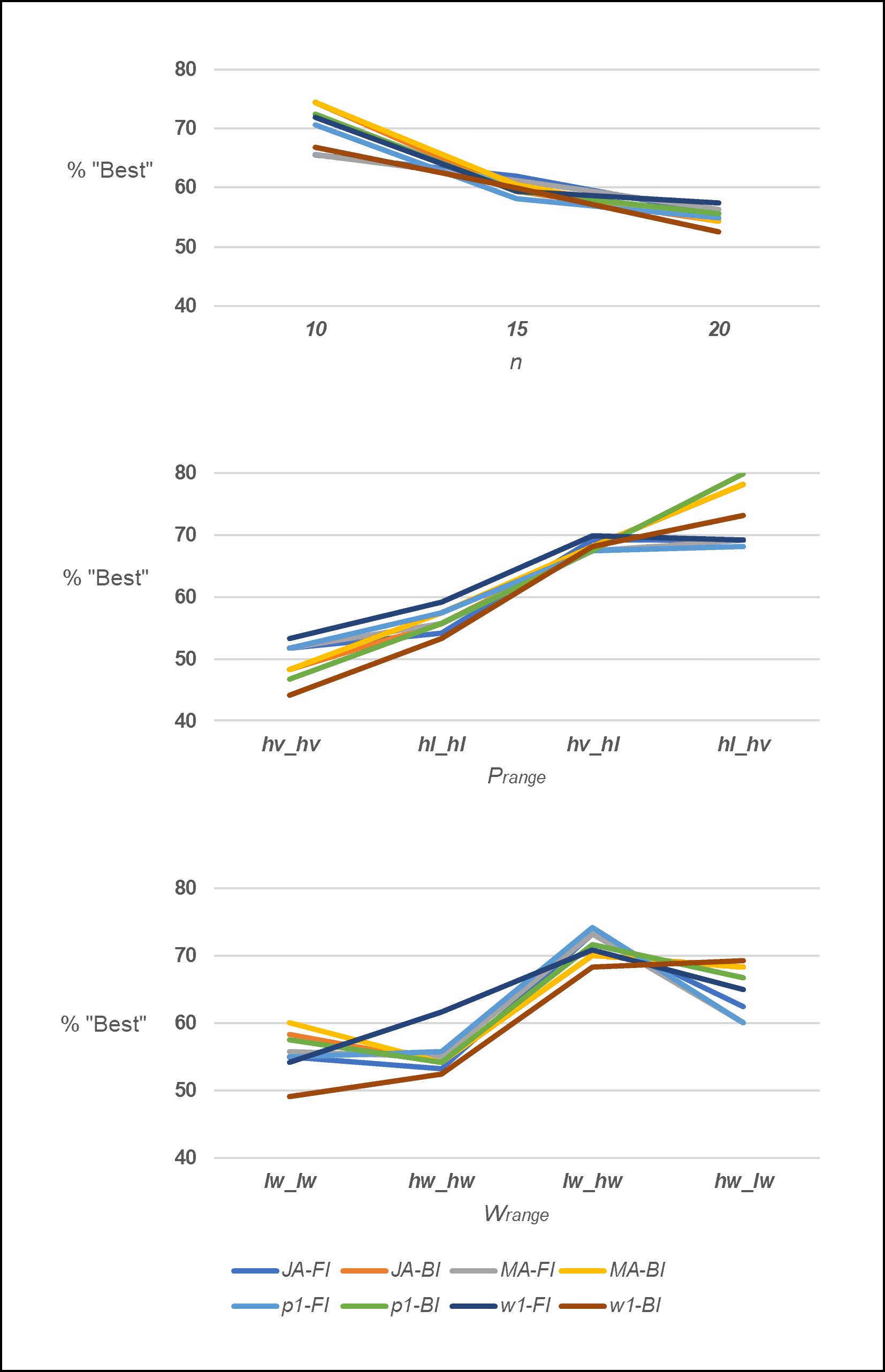
The results related to experimental factor 𝑤range are similar as heuristic performance depends on the specific level. The level hw_hw (where both machines deteriorate at the high level) is prominent given the highly notable difference in performance between the dominant heuristic (w1-FI) and the rest.
Table 7 presents the error characteristics when the heuristic does not find the best solution
Table 7 Mean and maximum error% for instances versus the “best” makespan solution
| Heuristic | JA FI | JA BI | MA FI | MA BI | p1 FI | p1 BI | w1 FI | w1 BI |
|---|---|---|---|---|---|---|---|---|
| Mean | 0.69 | 0.50 | 0.68 | 0.49 | 0.60 | 0.48 | 0.57 | 0.73 |
| Max | 6.19 | 3.54 | 6.19 | 3.31 | 6.22 | 3.31 | 6.09 | 5.62 |
(𝑒𝑟𝑟𝑜𝑟% = (1 - 𝑐 max [heuristic ]⁄ 𝑐 max [best found by al heuristic ])⨯100). Heuristic p1-BI, a heuristic that does not dominate under any of the experimental levels is the best performer in terms of the mean and the maximum error, although only surpassing the best performing MA-BI heuristic by a very small amount. In this case, the difference in performance among the heuristics is not as notable as in the optimal benchmark experiments. Based on the complete set of experiments it is concluded that heuristic MA-BI is the best performer for the makespan criteria.
3.3 Tardiness Results
Table 8 presents for each experimental level the average tardiness and the percentage of times that at least one of the heuristics found the optimal solution. At least one of the heuristics found the optimal solution in all but one instance, a 99.9% success rate (959 out of 960). The heuristics provide an excellent approximation to the optimal within the analyzed experimental structure.
Table 8 Mean average tardiness and % of optimal solutions found by at least one heuristic
| 𝑡 ave | % optimal | ||
|---|---|---|---|
| θ | 1 | 29.2 | 100 |
| 1.5 | 50.7 | 100 | |
| 2 | 83.5 | 99.7 | |
| 𝑛 | 6 | 50.9 | 100. |
| 8 | 58.1 | 99.8 | |
| 𝑝range | hv_hv | 43.4 | 100 |
| hl_hl | 56.8 | 99.6 | |
| hv_hl | 53.6 | 100 | |
| hl_hv | 64.3 | 100 | |
| 𝑤range | lw_lw | 41.6 | 99.6 |
| hw_hw | 66.8 | 100 | |
| lw_hw | 55.9 | 100 | |
| hw_lw | 53.6 | 100 | |
| Overall | 54.5 | 99.9 |
The set of heuristics included in the average tardiness analysis are different than in the makespan analysis based on the relative performance of the complete set of heuristics for this criterion, noting in this case there are 22 relevant heuristics. Table 9 presents the percentage of times each heuristic generated the optimal solution. The best two overall performers are p1-FI and d-FI which generated 88.9% and 88.2% of the optimal solutions, respectively. Heuristic p1-FI outperformed all others in 7 experimental levels, while d-FI outperformed all others in 3 experimental levels. Five of the heuristics dominate in at least one level. As it is the case in the makespan criteria for the optimal benchmark experiments, none of the initial job ordering heuristic dominates across the complete set, but for these experiments the FI improvement approach outperforms the BI approach.
Table 9 Percentage of the optimal average tardiness solutions generated by a heuristic
| Heuristic | WA | d | d | s | p1 | p1 | p2 | w1 | |
|---|---|---|---|---|---|---|---|---|---|
| FI | FI | BI | FI | FI | BI | FI | FI | ||
| θ | 1 | 95.3 | 96.9 | 94.7 | 96.3 | 96.9 | 90.9 | 96.3 | 95.0 |
| 1.5 | 86.9 | 87.2 | 88.4 | 86.3 | 88.1 | 80.6 | 88.4 | 88.8 | |
| 2 | 78.4 | 80.6 | 78.8 | 78.4 | 81.6 | 78.8 | 79.7 | 80.3 | |
| 𝑛 | 6 | 90.2 | 90.6 | 91.5 | 89.8 | 91.7 | 87.1 | 90.4 | 89.6 |
| 8 | 83.5 | 85.8 | 83.1 | 84.2 | 86.0 | 79.8 | 85.8 | 86.5 | |
| 𝑝range | hv_hv | 79.2 | 82.5 | 81.3 | 77.5 | 82.9 | 75.4 | 80.0 | 81.3 |
| hl_hl | 91.7 | 90.0 | 90.0 | 90.8 | 92.9 | 86.7 | 92.9 | 92.1 | |
| hv_hl | 86.7 | 90.4 | 87.5 | 89.6 | 88.8 | 78.3 | 89.2 | 88.3 | |
| hl_hv | 90.0 | 90.0 | 90.4 | 90.0 | 90.8 | 93.3 | 90.4 | 90.4 | |
| 𝑤range | lw_lw | 85.4 | 92.5 | 87.9 | 88.8 | 87.5 | 81.7 | 88.8 | 88.8 |
| hw_hw | 84.6 | 85.0 | 85.4 | 83.8 | 86.7 | 86.7 | 88.3 | 85.4 | |
| lw_hw | 85.0 | 84.2 | 83.8 | 85.0 | 88.3 | 77.1 | 85.4 | 85.0 | |
| hw_lw | 92.5 | 91.3 | 92.1 | 90.4 | 92.9 | 88.3 | 90.0 | 92.9 | |
| Overall | 86.9 | 88.2 | 87.3 | 87.0 | 88.9 | 83.4 | 88.1 | 88.0 |
Table 10 presents the mean and maximum error versus the optimal for those instances where the heuristic did not find the optimal solution. Heuristic d-FI provides the smallest average error at 4.6% and ties for the smallest maximum error with 40.3%. The second heuristic that considers the due date parameter in the ordering process, s-FI, ties with d-FI as the best overall performer for the maximum error. These results are notably different than those obtained for the makespan criteria where the mean error is smaller than 1.04 % and the maximum is less than 12.5%.
Table 10 Mean and maximum error% versus optimal.
| Heuristic | WA | d | d | s | p1 | p1 | p2 | w1 |
|---|---|---|---|---|---|---|---|---|
| FI | FI | BI | FI | FI | BI | FI | FI | |
| Mean | 7.6 | 4.6 | 6.0 | 5.7 | 6.0 | 13.1 | 6.6 | 7.2 |
| Max | 124.2 | 40.3 | 59.2 | 40.3 | 71.8 | 182.9 | 124.2 | 120.5 |
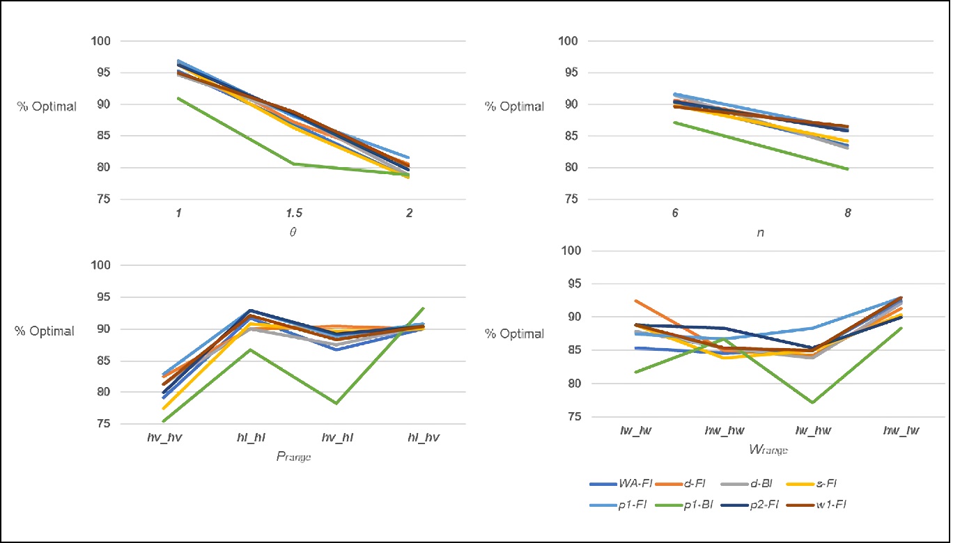
Figure 5 shows heuristic performance per experimental factor for the percentage of optimal solutions found. The overall performance decreases as the number of jobs and the due date tightness ratio factors (𝑛 and θ) increase. It is noted that heuristic p1-BI performs poorly for most of the levels for those two experimental factors. As in the makespan experiments, the relative performance of the heuristic changed notably at the different levels of the 𝑝range and 𝑤range factors. It is noted that for 𝑝range, heuristic p1-BI is the worst performer for three out of the four experimental levels, but for level hl_hv this heuristic is the best performer. For the 𝑤range parameter it is worth mentioning the relatively high-performance level of heuristics d-FI and p2-F1 for experimental levels lw_lw and hw_hw respectively.
The percentage of instances per experimental level where a heuristic generated the best average tardiness solution for the relative benchmark experiments is presented in Table 11. For these experiments, s-FI is the best overall performer generating 62.6% of the best solutions. The two runner ups in terms of overall performance are p2-FI and w1-FI. As in the previous cases, multiple heuristics dominate at least one experimental level, thus no dominant heuristic can be determined. In line with the previous results, the FI improvement heuristic does outperform the BI approach. The mean and maximum errors are presented in Table 12. As in the makespan case, a heuristic that does not dominate under any of the experimental levels is the best performer in terms of the mean and the maximum error, heuristic WA-FI. If having a small error and avoiding the maximum error is an important element of heuristic selection, heuristic WA-FI is the clear best overall performer.
Table 11 Percentage of the “best” average tardiness solutions generated by a heuristic
| Heuristic | WA | d | d | s | p1 | p1 | p2 | w1 | |
|---|---|---|---|---|---|---|---|---|---|
| FI | FI | BI | FI | FI | BI | FI | FI | ||
| 𝑛 | 1 | 79.4 | 79.0 | 79.4 | 80.8 | 77.9 | 66.5 | 79.2 | 79.4 |
| 1.5 | 56.9 | 59.6 | 53.3 | 59.6 | 57.5 | 54.6 | 56.7 | 57.3 | |
| 2 | 47.5 | 45.4 | 42.3 | 47.3 | 49.6 | 39.8 | 49.8 | 49.2 | |
| 10 | 79.8 | 79.4 | 77.7 | 78.1 | 80.6 | 72.3 | 80.0 | 79.6 | |
| 15 | 61.7 | 61.7 | 58.1 | 62.5 | 61.9 | 50.4 | 60.0 | 62.1 | |
| 20 | 42.3 | 42.9 | 39.2 | 47.1 | 42.5 | 38.1 | 45.6 | 44.2 | |
| 𝑝range | hv_hv | 48.3 | 48.9 | 48.9 | 48.9 | 50.6 | 37.8 | 51.9 | 49.7 |
| hl_hl | 65.3 | 65.3 | 62.2 | 66.9 | 65.0 | 62.2 | 67.5 | 67.2 | |
| hv_hl | 66.4 | 69.2 | 62.8 | 68.9 | 66.7 | 53.3 | 63.1 | 65.3 | |
| hl_hv | 65.0 | 61.9 | 59.4 | 65.6 | 64.4 | 61.1 | 65.0 | 65.6 | |
| lw_lw | 68.9 | 68.3 | 67.8 | 70.0 | 69.7 | 60.6 | 71.1 | 71.4 | |
| hw_hw | 52.2 | 53.6 | 47.5 | 53.1 | 55.3 | 46.7 | 52.2 | 56.4 | |
| lw_hw | 60.3 | 60.8 | 56.7 | 60.8 | 59.7 | 51.7 | 60.8 | 59.2 | |
| hw_lw | 63.6 | 62.5 | 61.4 | 66.4 | 61.9 | 55.6 | 63.3 | 60.8 | |
| Overall | 61.3 | 61.3 | 58.3 | 62.6 | 61.7 | 53.6 | 61.9 | 61.9 |
Table 12 Mean and maximum error for instances versus the “best” average tardiness solution
| Heuristic | WA | d | d | s | p1 | p1 | p2 | w1 |
|---|---|---|---|---|---|---|---|---|
| FI | FI | BI | FI | FI | BI | FI | FI | |
| Mean | 2.74 | 2.85 | 3.74 | 3.22 | 3.10 | 6.79 | 2.91 | 2.79 |
| Max | 37.5 | 50.8 | 65.8 | 77.3 | 103.7 | 201.0 | 50.8 | 50.8 |
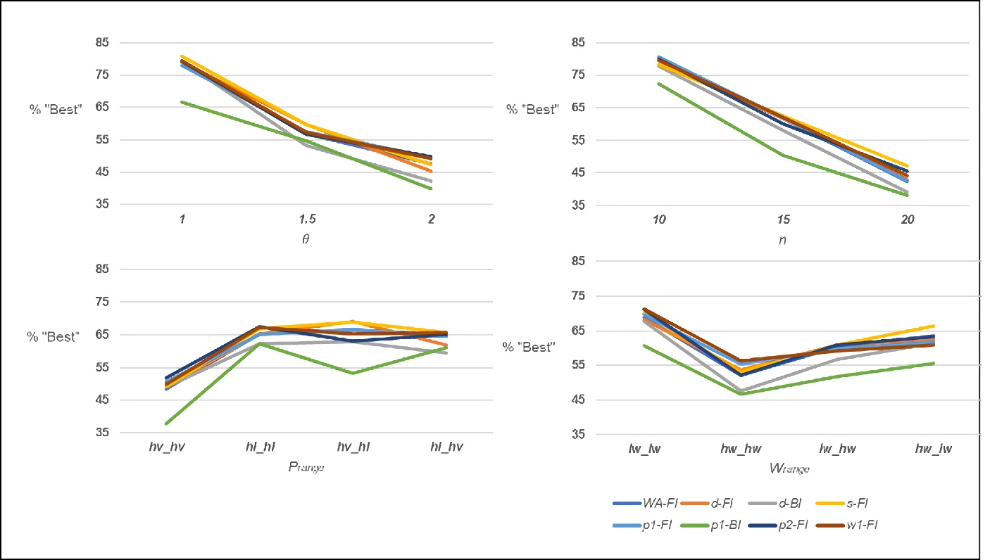
The tardiness results by experimental factor for the percent of “best” solutions found are illustrated in Figure 6. The effects are similar to those observed when evaluating heuristic performance versus the optimal solutions, although the effects more remarkable. For example, at θ = 1 and 𝑛 = 10, the percent found by the heuristics was in the 65-85% range, while at θ = 2 and 𝑛 = 20, the range is 35 to 55%. It is noted that this does not indicate an error versus the optimal as this value is unknown, but rather the inability of the heuristics to match each other’s performance. As in previous experiments, heuristic performance is affected by both 𝑝range and 𝑤range, and while no heuristic stands out as an excellent performer at particular levels of these factors, heuristic p1-BI stands out as one that is almost always outperformed.
This paper introduced a set of efficient heuristic approaches for solving the two-machine permutation flowshop problems while considering machine deterioration. The heuristic performance is assessed under two independent objectives: minimization of the makespan and minimization of the average tardiness. In the case of makespan minimization, eighteen heuristic approaches were developed based on different job characteristics. Similarly, a total of twenty-two heuristic approaches were elaborated when considering average tardiness minimization. A comprehensive experimental design was carried out considering variation of different experimental factors such as the number of jobs, the range of process time, the range of wear/deterioration rate, and the congestion ratio.
The experimental factor ‘number of jobs’ has a significant impact in the problem complexity. Hence, this factor was considered at two size levels. The first level determined the optimal benchmark experiments where the heuristic performance was evaluated versus the optimal solution. The relative benchmark experiments were defined by the second level. In this case, the heuristic performance was compared against the best-found solution.
The results from the optimal benchmark experiments exhibited a 98.1% and 99.9% heuristics overall success rate when considering makespan and average tardiness minimization, respectively. As expected, the results show that the success factor decreases as the number of jobs increases. However, the success rate was nearly 100% when the process time and wear/deterioration rate presented similar levels of variation at both machines. The top overall performers for makespan minimization were MA-BI and JA-BI, which found 83.8% and 83.4% of the optimal solutions respectively. Furthermore, MA-BI and JA-BI had a mean error of 0.45% and 0.46% respectively. In the case of average tardiness minimization, the best two overall performers were p1-FI and d-FI, which generated 88.9% and 88.2% of the optimal solutions, respectively. Heuristic d-FI provided the overall smallest average error at 4.6%; in contrast, p1-FI had an average error of 6%.
The relative benchmark experiments were compared versus the best-found solution. In alignment with the previous results, the heuristic performance decreases as the number of jobs increases. The top overall performers for makespan minimization were MA-BI and w1-FI, which found 63.1% and 62.9% of the ‘best’ solutions, respectively. However, p1-BI had the smallest overall mean error at 0.48%. In the case of average tardiness minimization, the best three overall performers were s-FI, p2-FI, and w1-FI, which generated 62.6%, 61.9%, and 61.9% of the optimal solutions, respectively. Heuristic WA-FI provided the overall smallest average error at 2.74%; in contrast, s-FI had an average error of 3.22%.
Results showed that there is no heuristic that has full dominance in any combination of experimental factors. Furthermore, the different experimental settings had a notable role in the heuristic performance suggesting that all of them should be utilized when solving real case instances. Immediate future research streams are as follows: 1) The consideration of maintenance events that could help to mitigate the undesirable effect of machine deterioration. 2) The extension of the presented approach to the ‘m’ machines flowshop problem. 3) The analysis of more complex interdependencies among the process time and wear/deterioration rate with different job sequences. For example, given materials and mechanical properties, a specific sequence of jobs could generate a different deterioration rate than if they are performed in another specific sequence. The implementation of the results learned in this research in applied production and industrial engineering settings could provide significant competitive advantages to the organizations by reducing the makespan, which is directly related to operational costs, and the average tardiness, which is directly related to customer service.

