


 Inglés (pdf)
 Articulo en XML
 Referencias del artículo
 Enviar articulo por email
 Citado por SciELO
  Citado por Google
  Similares en
SciELO
Similares en
SciELO  Similares en Google
 Permalink
Introduction
Atrial Fibrillation (AF) is the most common cardiac arrhythmia in clinical practice. Its global prevalence is around 2% in the community, around 5% in patients older than 60 years and 10% in people over 80 years old. AF is associated with reduced quality of life and also increases the risk of stroke and myocardial infarction. In Colombia, some studies show that the incidence and mortality of AF has increased especially in people over the age of 70 [1], [2].
AF is caused by various health complications. During an episode of AF, the contraction of the atria is asynchronous because of the fast firing of electrical impulses. The main characteristics of an AF episode are: The absence of a sinus P wave, irregular and fast ventricular contraction, presence of an abnormal and variable RR interval, atrial heart rate oscillates from to beats per minute (bpm) and narrow QRS complexes (< 120milliseconds) [1].
By using electrodes placed on the skin is possible to record the heart's electrical activity. A voltage vs time graph is known as an electrocardiogram (ECG signal). These electrical changes are a consequence of cardiac muscle depolarization followed by repolarization during each cardiac cycle (heartbeat). The ECG morphology contains important information about the conditions of the heart. Thus, the ECG signals are used to detect abnormalities in heart activity [3].
The ECG signals are interpreted manually by cardiologists in order to detect cardiac abnormalities. The detection of AF demands to analyze long recordings because of its paroxysmal nature. These analyses are time-consuming, expensive, and sometimes could be subjective. Figure 1 shows typical ECG signals. The blue representation is a normal ECG signal and the other (red) representation is an Atrial Fibrillation ECG.
Note that the abnormal activity of the atria produces variations in heart rate and a faster ventricular response, although there is also the opposite case, where the ventricular response becomes slower.
The AF is generally asymptomatic or shows nonspecific symptoms [5]. However, several medical reports call attention to the importance of early diagnosis in order to start an early treatment [6], [7]. However, these early diagnostics are quite difficult to do in countries like Colombia, where there is an irregular distribution of cardiologists around the country. For example, more than 80% of cardiologists are localized only in seven of the main cities in Colombia [8]. Thus, the intermediate cities, small towns, and rural zones do not have the possibility to access an early cardiology service.
Convolution Neural Networks (CNN) have been used to detect cardiac arrhythmias. In [9] a 1-D CNN approach is used, which classifies the ECG signal for the detection of ventricular ectopic beats and supraventricular ectopic beats with a very high accuracy.
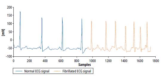
Source: Self-made.
Fig. 1: Signals from MIT BIH AF Database. Normal ECG, Atrial Fibrillation ECG. [4]
The [10] Georgia Institute of Technology, in Atlanta has developed a CNN approach to detect AF. In this work, the cardiac signals are recorded by a Pulsatile photoplethysmographic sensor. The approach uses a Wavelet Transform before feeding the CNN. Finally, a multinomial regression is used to establish the presence or absence of an episode of AF. This approach obtained of accuracy. In [11] signal quality index SQI technique was combined with CNN followed by a post-processing feature-based approach to classify AF. The accuracy for the PhysioNet/CinC database was.
This work is part of a macro project that seeks to develop a medical device, which is based on a CNN. The macro project aims at offering an alternative for diagnosis in areas where there is no cardiology service.
The aim is to find a suitable CNN model that could be later implemented in hardware. We apply diverse techniques regarding batch, learning rate, and optimizer function in order to improve the accuracy, sensitivity, specificity, and precision of the network. Our proposed model achieves an accuracy of , a specificity of , a sensitivity of and a precision of for specific patients. We used the MIT BIH Atrial Fibrillation Database [4]. Moreover, the proposed model performs the best sensitivity at a lower computational cost.
The rest of this paper is organized as follows: Section 2 shows a description of the database. Section 3 introduces the convolutional neural networks. In Section 4, we develop the training methodology and the tests done for different topologies regarding optimization techniques. The results are summarized in Section 5. Finally, the conclusions close the article.
Database
We use ECG signals from a free public arrhythmia database called MIT BIH Atrial Fibrillation Database [4]. This database includes 25 long-term ECG recordings, which were sampled at 250 samples per second with a 12 bits resolution in a range of . The recordings were made at Beth Israel Hospital in Boston, among people with atrial fibrillation (AF), which include more than 300 episodes of AF. The database has non-numerical annotations, which are given according to a convention. An indicates an AF episode and a indicates a normal episode. The annotations were taken when there was a change of state, either from to or vice versa.
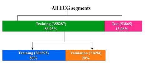
A pre-label function was created to label 500-sample segments. Then, each segment was normalized from 0 to 1. Finally, the normalized segments were randomized to guarantee the performance of the algorithm. The distributions of database were made by the following terms:
■ 20 patients for training equivalent to 358287 segments (86.93%)
► 286593 segments for training (80%)
► 71694 segments for training (20%)
■ 3 patients for test equivalent to 53865 segments (13.06%)
Convolutional Neural Networks (CNN)
To the best of our knowledge, Japanese scientist Kunihiko Fukushima published the first CNN model in 1980 [12]. Then, the French scientist Yann LeCun improved this first model in 1988 [13]. LeCun's model uses three types of layers: Convolutional, sub-sampling and fully connected layers. Convolutional layers extract features from the input image. Sub-sampling layers reduce both spatial size and computational complexity. Finally, the Fully connected layers classify the data. CNN has been implemented in various applications such as: object recognition [14], [15], handwriting classification [16], [17] and image classification [3], [18], [19], to name a few.
Recently some works have used the CNNs as a diagnostic tool of diseases such as heart attacks [20], colon cancer [18], melanoma [21], Alzheimer [22], cardiac arrhythmia's [3] and hemorrhage detection [19].
Figure 3 shows the basic configuration of a convolutional neural network, which is the combination of three basic ideas. First the Convolution Layers, which extract features of the data and reduce the number of weights. Second, the pooling layers (also known as subsampling layers), which reduce the number of connections. Finally, the fully connected layers, which develop the classification process. Note that every layer of convolution is coupled with a subsampling layer and an activation function, before reaching the fully connected layers.

Selecting the CNN architecture: A hardware point of view.
As mentioned before, several computational CNN architectures have been developed [3], [10], [11], [20]; they focus on achieving higher accuracy. However, these works do not take into account issues regarding hardware and power consumption. We are interested in the development of a computational CNN architecture that achieves the highest accuracy using the least number of parameters possible. Reducing the number of parameters allows the reduction of power consumption.
The possible models for the solution of problem are:
■ Dense Neural Network model (Multilayer Perceptron)
■ Convolutional Neural Network model
► 1D (Deep Learning)
► 2D (Machine Learning): FFT / SFT / Wavelet
The kind of architecture selected is the Convolutional Neural Network in 1 dimension (CNN 1D) because the documentation available proves that it offers excellent efficiency for the time series [9]. Due to the fact that the heartbeat can be interpreted as a time series, it's more feasible to obtain good results. For the architecture selection, we tried three different topologies, therefore, a test was made in a preliminary stage, using a part of the database and the same parameters for the optimization process and regularization techniques in the three proposals, to determine the most efficient in terms of accuracy. In brief, the advantages of the 1D CNN model are:
■ They perform extraction and reduction of characteristics.
■ They allow reducing the bidimensionality of the problems.
■ Decrease in pre-processing requirements.
■ The particular signal to be treated for the problem in its natural form is a linear sequence of data.
It represents fewer parameters and reduces the number of operations compared to a 2D network, which is advantageous to reduce the computational cost, memory and energy of the project in future implementations in FPGA.
We developed three CNN architectures that were implemented from low complexity to high complexity, in order to establish better results with the lowest complexity and lowest number of parameters possible.
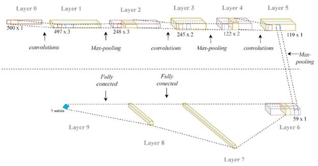
Figure 4 shows architecture 1 that consists of 9 layers distributed as follows:
■ Convolutional layer, with 3 kernels of size 4.
■ Max-pooling layers of with stride = 2
■ Convolutional layer, with 2 kernels of size 4.
■ Max-pooling layers of with stride = 2
■ Convolutional layer, with 1 kernel of size 4.
■ Max-pooling layers of with stride = 2
■ Fully-connected flatten layer
■ Fully-connected layer with 10 neurons
■ Fully-connected layer with 1 neuron
■ RELU activation function, used for the convolutional layers and middle fully-connected layer.
■ Sigmoid activation function used for the output layer.
Architecture 2 consists of 9 layers in total, which are distributed as follows:
■ Convolutional layer, with 3 kernels of size 15.
■ Max-pooling layers of with stride = 2
■ Convolutional layer, with 5 kernels of size 10.
■ Max-pooling layers of with stride = 2
■ Convolutional layer, with 10 kernels of size 10.
■ Max-pooling layers of with stride = 2
■ Fully-connected flatten layer
■ Fully-connected layer with 10 neurons
■ Fully-connected layer with 1 neuron
■ RELU activation function used for the convolutional layers and middle fully-connected layer.
■ Sigmoid activation function used for the output layer.
Architecture 3 consists of 11 layers in total, which are distributed as follows:
■ Convolutional layer, with 3 kernels of size 27.
■ Max-pooling layers of with stride = 2
■ Convolutional layer, with 10 kernels of size 14.
■ Max-pooling layers of with stride = 2
■ Convolutional layer, with 10 kernels of size 3.
■ Max-pooling layers of with stride = 2
■ Convolutional layer, with 10 kernels of size 4.
■ Max-pooling layers of with stride = 2
■ Fully-connected flatten layer
■ Fully-connected layer with 30 neurons
■ Fully-connected layer with 10 neurons
■ Fully-connected layer with 1 neuron
■ RELU activation function used for the convolutional layers and the two middle fully-connected layers.
■ Sigmoid activation function used for the output layer.
Table 1 summarizes the composition of layers and their trainable parameters. This table indicates the size of the output feature maps of each layer. Note that, Max-pooling (sub-sampling) layers do not have trainable parameters.
Table 1 Architecture comparison
| Architecture 1 | Architecture 2 | Architecture 3 | ||||||
|---|---|---|---|---|---|---|---|---|
| Layer type | Output shape | # parameters | Layer type | Output shape | # parameters | Layer type | Output shape | # parameters |
| in | (500,1) | 0 | in | (500,1) | 0 | in | (500,1) | 0 |
| convolutional | (497,3) | 15 | convolutional | (486,3) | 48 | convolutional | (474,3) | 84 |
| max pooling | (248,3) | 0 | max pooling | (243,3) | 0 | max pooling | (273,3) | 0 |
| convolutional | (245,2) | 26 | convolutional | (234,5) | 155 | convolutional | (224,10) | 430 |
| max pooling | (122,2) | 0 | max pooling | (117,5) | 0 | max pooling | (112,10) | 0 |
| convolutional | (119,1) | 9 | convolutional | (108,10) | 510 | convolutional | (110,10) | 310 |
| max pooling | (59,1) | 0 | max pooling | (54,10) | 0 | max pooling | (55,10) | 0 |
| flatten* | 59 | 0 | flatten* | 540 | 0 | convolutional | (52,10) | 410 |
| dense | 10 | 600 | dense | 10 | 5410 | max pooling | (26,10) | 0 |
| dense | 1 | 11 | dense | 1 | 11 | flatten* | 260 | 0 |
| dense | 30 | 7830 | ||||||
| dense | 10 | 310 | ||||||
| dense | 1 | 11 | ||||||
Source: Self-made.
Training the architectures
We trained architecture 1 with the following algorithm:
■ Optimization method: SGD
■ Loss evaluation method: Binary cross entropy
■ Activation function of the middle layers: relu
■ Activation function of the final layer: Sigmoid
■ Epochs: 40
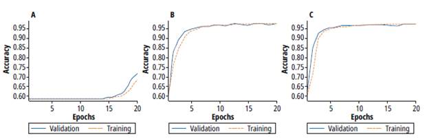
Figure 5 shows the accuracy results for training (orange line) and validation (blue) processes of the architectures 1, 2 and 3 respectively.
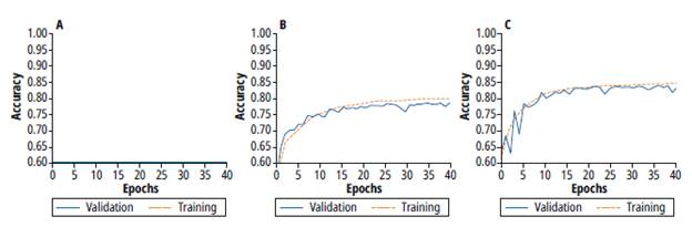
Source: Self-made.
Fig. 5 Training and validation process for a) Architecture 1 b) Architecture 2 c) Architecture 3
Architecture 1 does not increase accuracy during the training process. The constant behavior of the accuracy is due to the few amounts of parameters. Besides, there is a high bias and high variance. On the other hand, architecture 2 achieves better accuracy than architecture 1. However, during the validation process, a high variance and noise validation are observed. Finally, architecture 3 achieves better accuracy levels. However, there is still a high variance in this architecture, which demands to apply additional techniques to reduce this variance. Table 2 summarizes accuracy results for the three architectures. Besides, this table also shows the number of trainable parameters, which are related to the amount of memory required during the inference process.
Testing different batch values
We performed a test with different batch values for architecture 3, which achieved better accuracy in the previous test. This test is made to determine a value that improves the accuracy level for the training and validation process. Small batch values imply more operations in the calculus of gradient, but high values cause higher error, regarding the validation rate. The batch values used were 10, 15, 20, 25, 50, 100 and 200. Training and testing processes were performed for each batch value with the following parameters:
■ Optimization method: SGD
■ Loss evaluation method: binary cross entropy
■ Activation function of the middle layers: RELU
■ Activation function of the final layer: Sigmoid
■ Epochs: 40
Figure 6 shows the results for the training accuracy of different batch values. Notice for values over 50, the learning process is stable. Due exist multiple values that improve the training process, criteria for the selection of value is the tendency of the process with less variance. Table 3 shows the result of the analysis of variance in each test. Therefore, regarding the lowest variance, the batch value selected for the next test is 100.
Table 3 Statistical variance VS Batch size
| Batch | 10 | 25 | 50 | 100 | 200 |
| Variance | 0.7498e-03 | 0.3783e-03 | 0.2919e-03 | 0.2213e-03 | 0.4404e-03 |
Source: Self-made.
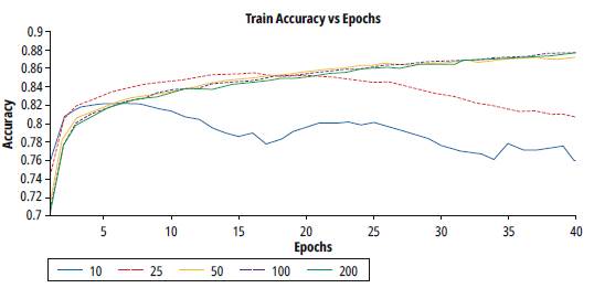
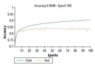
Figure 7 shows the results of training and validation accuracy for a batch value of 100. Note that there is an improvement in the training process, however, the validation process stops the generalization from epoch 10.
Testing different learning rate values
For improving the response regarding learning rate values, a test was performed using SGD optimizer, and batch value for previous test. A test was performed using SGD optimizer to improve the response regarding learning rate values, and the obtained batch value from the previous test.
Several learning rate values were used during the testing process, but this section summarizes just the range of the best results. The training and testing parameters used were:
■ Optimization method: SGD
■ Loss evaluation method: binary cross entropy
■ Activation function of the middle layers: RELU
■ Activation function of the final layer: Sigmoid
■ Epochs: 100
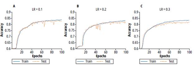
Figure 8 shows the training and validation processes for learning rate values of 0.1, 0.2 and 0.3. Note that for values 0.1 and 0.2 the learning process takes more epochs but evidences a lower variance. On the other hand, for a learning rate of 0.3, the training process takes fewer epochs but a higher variance. Thus, a learning rate value of 0.1 was selected.
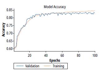
A new test was performed with the learning rate value selected. This test was performed with the calculated parameters from the previous tests. In this case, we change the learning rate epoch by epoch with a constant decay factor. Figure 9 summarizes the results of this test. Note that the accuracy reached is similar to the previous test, but it takes a few numbers of epochs. However, the variance is increased when the number of epochs is over 60.
Testing different optimizers
We tested 3 different optimizers. The tests keep the learning rate and batch values calculated in the previous test. Figure 10 shows the training process using three optimizers, a) SGD, b) RMSPROP and c) ADAM. For SGD optimizer, note that the training process takes a lot of epochs to begin the learning process, which means more computational cost. Figure 10 b) shows the training process using a RMSPROP Optimizer. In this case, the training process takes fewer epochs, and reaches stability at 10 epochs, with low variance (less than 0.36%). In spite of the similarity of the SGD and RMSPROP algorithms, figure 10 b) shows the advantages of the RMSPROP regarding the modification of the velocity function produced by the hyperparameter. Figure 10 c) shows the training using ADAM Optimizer. The training process increases faster than in SGD and RMSPROP, and the accuracy that is achieved is similar to RMSPROP. Besides, the trends for both RMSPROP and ADAM optimizers are similar.
Source: Self-made.
Fig. 10: Training and validation process for different optimizers a) SGD b) RMSPROP c) ADAM
Table 4 Train and Validation Accuracy Vs Learning Rate
| LR | 0.1 | 0.2 | 0.3 |
| train | 83.91% | 83.19% | 83.59% |
| validation | 83.39% | 82.35% | 82.24% |
Source: Self-made.
Table 5 summarizes the accuracy achieved by each optimizer, for both train and validation processes. Note that both RMSPROP and ADAM optimizers achieve similar accuracy in training processes. Regarding the lower computational cost in the training process, RMSPROP shows better efficacy, considering that the calculus of sensitivity is less complex.
Results
For the training process, we use an Intel Core i5 with 2.9 GHz, and 8 Gb of RAM memory. The description language used was Python 3.5 in the Jupyter notebook application. Python environment was created using Anaconda Navigator with Tensor Flow Back-end and the Keras libraries for AI.
Figure 11 shows the confusion matrix for the RMSPROP-based learning algorithm for a specific patient. This matrix shows: the normal signal well and wrongly classified, fibrillated signals well and wrongly classified, the accuracy, the specificity, the sensitivity, true positives, true negatives, false positives, false negatives and precision.
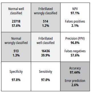
Source: Self-made
Fig. 11: Confusion matrix for the RMSPROP-based learning algorithm for specific patient.
In this case, the sensitivity is measured when all the input signals are fibrillated (positive condition). The value of sensitivity is the rate between the number of fibrillated signals well classified over the total of input signals. The specificity is as the sensitivity case but for normal signals (negative condition).
The Positive Predicted Values (PPV) are the rate between the true positives (True Fibrillated signals), and the number of values predicted as positive. The Negative Predicted Values (NPV) are the rate similar to PPV, but with the negative signals (Normal signals). The False Positives Value are the rate between the false positive (Normal signals predicted as Fibrillated) and the number of condition negative signals (True normal signals). The false Negative Value is the rate between the false negative signals (Fibrillated predicted as normal) and the total of true positive conditions.
We developed two tests, one for a specific patient and another one for a general group, both using k-fold validation, 7 random selection of patients in the dev-set group. Table 6 summarizes the main results for the confusion matrix for the three optimizers used. Note that the ADAM reaches the best specificity (negative condition - normal signals). On the other hand, the RMSPROP achieves the best values for accuracy, sensitivity, and precision. It is important to note that in the case of disease diagnosis, one of the most important statistical values is the sensitivity (positive condition - fibrillated signals).
Conclusions
We have developed a CNN model to automatically identify AF from 2-second ECG signals (500 samples). We tested several batches and learning rate values and three different optimizers. Our results suggest that a batch and learning rate of 100 and 0.1, respectively, improve the validation accuracy. On the other hand, the RMSPROP is the best optimizer in this case, because of its matrix confusion results and its low computational cost. We aim to use this model in future work, which will focus on the implementation of a CNN-based portable device for automatic detection of AF in Colombia.

