


 Inglés (pdf)
 Articulo en XML
 Referencias del artículo
 Enviar articulo por email
 Citado por SciELO
  Citado por Google
  Similares en
SciELO
Similares en
SciELO  Similares en Google
 Permalink
Introduction
The concept of modeling terrestrial surfaces has been the object of topography study and has been continuously investigated and advanced during the last years [1]-[3]. LiDAR technology is a remote sensing system used to model topographic surfaces through multiple returns of laser pulses combined with GNSS location data. It provides a great density of terrain points and surface characteristics, like vegetation, water, and artificial structures. LiDAR has been used in various areas, such as hydrological modeling [4], [5], glacier monitoring [6],[7], forest characterization [8], and urban modeling [9], [10]; however, this technology focuses primarily on the characterization of complex traits of the terrestrial surface [11]. LiDAR offers a precise way of producing digital elevation models (DEM) for high-accuracy mapping applications through point clouds with levels of detail that other surveying technologies have not been able to equal.
Te search for an increasingly detailed representation of the attributes of the terrain converges on high-density LiDAR data sets and, therefore, on the complications of excessive consumption of processing, storage, and information manipulation time, leading to thinking about a reduction in the size of the sets; in that sense, it is necessary to select the lowest number of points that preserve the elements of topographic description. Given that there is no selection of the sampling density for different areas during a data collection mission, some terrains can be oversampled [12]. Diverse strategies have been proposed to treat large data sets without compromising their accuracy. Duan et al. [13] proposed an adaptive clustering method based on principal component analysis (PCA) to filter LiDAR point clouds. Hodgson and Bresnahan [14] indicated that the primary objective of specifying parameters to collect LiDAR data is to achieve high spatial density. Anderson et al. [15] evaluated the Kriging and idw interpolation techniques and the effect of the LiDAR data density on the statistical validation of linear interpolators, finding that Kriging yields slightly better results than idw; however, idw interpolation is computationally lighter and provides rapid interpolation of the topographic surface. Hodgson et al. [16] found that the sampling density for the LiDAR terrain returns varied in the categories of soil coverage; the results indicated a significant increase of the error in the coverage of bushes and shrubs. Furthermore, they found that only the elevations covered by low grasslands increased the error as a slope function. Later, Anderson et al. [15] evaluated the data reduction capacity generating dem for five sampling subsets, using the ANUDEM interpolator and three grid sizes. They found that when producing 30-m dem, LiDAR datasets could be reduced to 10 % of their original data density without statistically altering the dem produced.
Given that models are an approximate description of reality and are constructed by applying assumptions, they are never exact and, hence, susceptible to containing errors of random, systematic nature, or both. These errors must be evaluated to minimize their effects or correct them when understanding their origin. Sources can be diverse: insufficiency of points, incorrect distribution in their location, poor selection of interpolation algorithms, terrain complexity, or spatial resolution [17].
The grid size selection depends on two factors: the object of study-which is frequently measured as the quality of the results required as a function of the resolution-and the attributes of the source of data collection: accuracy, density, and distribution. According to Hengl [18], the resolution of the grid size can be related to the geometric disposition of the points due to the spatial trend pattern, through which the average spacing of points between the sampling data identifies the adequate grid size. Various criteria exist to define grid size; however, this work evaluated the models proposed by Hu, Tobler, and Hengl [18], [19], [20], which will be presented in the following section.
This research project used Kriging and row interpolators, both local types, based on Tobler's law [21]. row has demonstrated reliable results at different resolutions and relief characteristics; the results are ideal in high-density data with the regular spatial distribution. Kriging is widely used because it allows knowing the optimal search radius of neighbors from the variation among the data elevation as a function of its separation (semivariogram), provides unbiased estimation and minimum variance, and calculates the associated error for each estimated value. It does not use a simple mathematical function to represent the smoothed surface; in contrast, it recurs to a statistical function. It is ideal for dispersing data or data with irregular spatial distribution [22], [23]. Kriging is driven by Gaussian processes and estimates the mean value of the phenomenon, which means that the normal distribution is an assumption that must be fulfilled before its application [24].
This study, besides focusing on the effect of data reduction in the search for the density-volume ratio-which various authors cited have already proposed-seeks to conserve the sensitivity of the representation of the terrain in the function of three surface topographic descriptors: slope, curvature, and roughness, to improve the effectiveness of data processing in storage terms, and to achieve this objective, production is proposed using multiple DEMS with the division of original data in proportions of 100, 75, 50, 25, 10, and 1 % to apply the Kriging and row interpolators and measure their representation error with the cross-validation technique. This paper is organized as follows. In the first section, we describe the different datasets used to develop the project. Then, the modeling approach is explained. The second section presents the results of the experiments. Finally, discussion conclusions and recommendation research are given.
Materials and Methods
Study Area and Data
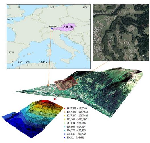
Schruns is a town in the city of Bludenz in the federal state of Vorarlberg. The geodetic coordinates of the city center are 47.08 ° N and 9.92 ° E. The terrain has a moderate inclination and steep slopes; the elevation variations range from 677 to 1218 m. The average slope of the area is 21.7°. Land use/ land cover classes include forest (42 %), grasslands (39 %), and buildings (19 %).
The Trimble Harrier 56 system acquired LiDAR raw data with a pulse repetition frequency of 160 kHz, maximum scan angle of 30 °, and average point density of 24 echos/m2. The data collection mission was conducted in August 2013 in Schruns. The study area was covered by six flight strips, each covering an area about 190 m across. The size of this dataset was 1.4 GB. The dataset contains a cloud of more than 55 million points and an area of 156 ha. The average spacing was 0.17 m. The information corresponding to the ground data indicates a separation average of 0.21 m and a volume of more than 32 million points. For visualization purposes, the input data was converted with the extension.LAS to.xyz using LAStools freely available at https://rapidlasso.com/lastools/. The LiDAR point cloud was generated using ArcGIS* (https://esri.com/), as shown in Fig. 1.
Method
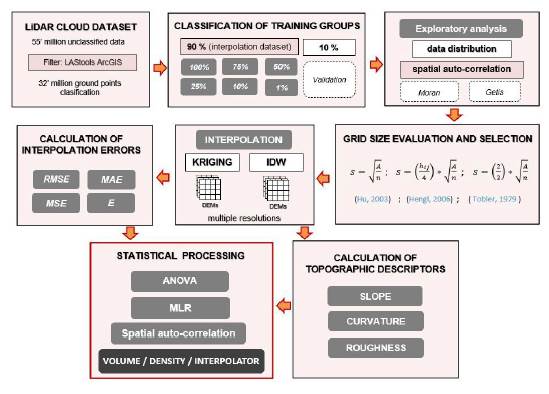
This Section is focused on the extraction of the parameters considered most relevant for modeling the effect of the density of LiDAR data without compromising the altimetric quality of the topographic representation. First, the 55 million measurement LiDAR dataset was filtered with LAStools, obtaining 32 million ground points. Then, they were randomly divided into two sets, the first with 90 % to build DEMS at different densities and grid sizes, the second with 10 % for validation. The grid size of the DEMS was defined by evaluating the Hu, Tobler, and Hengl models. Subsequently, Kriging and row interpolators were applied to obtain 72 surfaces from which the interpolation errors were derived. Finally, the errors were analyzed by multiple linear regression (MLR) and multifactor ANOVA to identify the influence of slope, curvature, and roughness on them (Fig. 2).
Exploratory Data Analysis
Descriptive, qualitative, and quantitative statistical analysis was performed to describe the trend of data distribution and its degree of dispersion to remove the presence of outliers, defining variables such as median, mode, quartiles, range, variation coefficient, histogram elaboration, and box and whisker diagrams.
Classification of Training Groups
When using ground points, a division was made into two subsets by random selection. In the first subset (calibration), 90 % of the data was obtained with which DEMS were produced at different relative densities in the following proportions: 100, 75, 50, 25, 10, and 1 %. The second subset corresponded to 10 % of the original data used as checkpoints to validate the information generated by the DEM created with the training data. For this purpose, cross-validation was used. The technique removes elevation values (temporarily), executes the interpolation algorithm, and estimates the values interpolated in the temporary withdrawal positions.
Analysis of Grid Size
When converting vector structures to raster to produce a DEM, interpolation techniques must be used to define the central value of each grid. In that sense, it is necessary to define the spatial resolution, which, as already exposed, affects the final quality of the DEM. To define the grid size, three models of different authors referred to in eq. (1), Hu, Tobler, and Hengl, were evaluated:
where, A, n, hij, and s, are area, sampling data, average spacing of points, and grid size, respectively.
Interpolation with Probabilistic and Deterministic Algorithms
Of the interpolation dataset, each sampling (100, 75, 50, 25, 10, and 1 %) was applied with the Kriging interpolator, minimizing the error variability through the fit of the experimental semivariogram to the theoretical models disposed of in the Geostatistical Analyst module by ArcGIS (spherical, linear exponential, or Gaussian). Interpolation was also conducted with IDW at different grid sizes in each sampling level to analyze the range of data variation and confront its results with the original data.
Calculation of the Interpolation Error
Comparison of predictions obtained from proposed interpolators was made using statistics; root-mean-square error (RMSE), mean absolute error (MAE), mean square error (MSE), and prediction effectiveness index (E). Analytical expressions of these indices can be found in Voltz and Webster [25] and Gotway et al. [26].
Topographic Descriptors
The slope, curvature, and roughness were calculated. The rationale for selecting these parameters is as follows: First, given its importance in anthropogenic processes such as earthwork calculations. Second, due to its usefulness in soil erosion and hydrological response, the processes define convexity, concavity, or superficial plain [27]. Third, because it points to the complexity of the terrain in terms of its undulation, indicating importance in biological and geological sciences [28]. Morphometric parameters were calculated with SAGA software, freely available at http://www.saga-gis.org/en/in-dex.html. The slope was reclassified according to the range and morphology of the terrain proposed by IGAC [29]. Curvature calculation used the model proposed by Dikau [30] based on the combination of convex, straight, and concave profiles. Roughness was calculated using the Riley, DeGloria, and Elliot model [31].
Statistical Processing of Data
To check the significance of the results produced, multifactor ANOVA was applied, relating the calculation of interpolation error by Kriging and IDW to the different resolutions proposed and the topographic descriptors slope, curvature, and roughness. MLR was used to identify the variability contribution introduced by one variable over another. Autocorrelation was measured through the Moran and Getis indices to characterize the behavior of elevations over the surface.
Results and Discussion
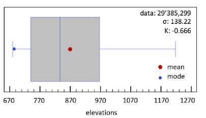
Univariate analysis was used to detect the statistical properties of the points. As inferred from Fig. 3, there is no data symmetry since the mean, median, and mode do not coincide in their values. The median and mode values are to the left of the mean; this distribution is assumed to have positive asymmetry, that is, the small data are abundant. Although the symmetry or lack of it does not guarantee normality, a pointing coefficient close to zero of mesokurtic type is; however, the kurtosis coefficient identifies the distribution as platykurtic type. A trend of data bias is evident toward the right, and the presence of atypical values is discarded.
Chi-squared and Kolmogorov-Smirnov tests were carried out to detect if the data adjusted to the usual trend, logistic or log-normal, given that these last two are positively biased functions with a high source of variability quite close to the Gaussian distribution. In both models, the probability, adjusting the data for any of these distributions was < 0.01.
Spatial autocorrelation was measured using the Moran index; its value was 0.96, indicating spatial grouping; this means that data within the sample share similar information in contiguous locations radiating through many spatial geographic units suggesting redundant information.
The Getis Ord index was calculated to identify the grouping level, which produced a value of 0.000061; the Z value of 25.98 shows positioning toward the right against the G observed, discarding the distribution randomness and ensuring that the data are highly grouped. During LiDAR data collection missions, scanning flight lines generally overlap, producing duplicity of points distributed irregularly. Besides, the plant coverage and the objects with which the sensor interacts generate unique optical properties, which is why soil coverage plays an important role, given that the points obtained are of high density and are configured in space almost uniformly. However, not every point helps produce the DEM; bodies of water, artificial objects, and the very structures of nature generate a different response when they interact with light rays, permitting to obtain too much or too little information on occasions.
Normality Conditions of Data Prior to Kriging Interpolation
Given that data were not normally distributed, data grouping was performed on the higher density training set (100 %). Initially, sampling was used with 5-m grid cells, extracting the value from the center. A subset of 62,500 points was obtained; then, the sample mean estimator was used, through which these were grouped into subsets of 200 data. The average value of each group was calculated, generating a final set of 313 data distributed normally. However, it made no sense to use this small dataset, considering that LiDAR is characterized by data with a large density of information and highly accurate results.
Subsequently, different types of transformation were tested: linear (standardization, punctual estimation) or nonlinear
 , which seeks to reduce the erratic behavior of the variogram models and make the continuity structure more evident [32]. The linear method produced a result not associated with normality; then, for the nonlinear transformation, considered ideal when the original variable has positive asymmetry, the results of the Chi-squared and Kolmogorov-Smirnov tests also did not indicate normality. Although the nonlinear transformations are helpful to force the sets into being more symmetrical, care must be taken, given that the retransformation of the data to the original variable tends to exaggerate any associated error with the interpolation, which is why after a transformation process, the characteristic to minimize the Kriging variance is lost. Application of the central limit concept would be very feasible and would guarantee data normality whenever the variable had a random spatial configuration, which would allow inferring that if the 1 % training set behaves normally with mean x̅ and variance σ
2
/n, all the other sets behave normally or asymptotically normal as
n
tends towards infinite.
, which seeks to reduce the erratic behavior of the variogram models and make the continuity structure more evident [32]. The linear method produced a result not associated with normality; then, for the nonlinear transformation, considered ideal when the original variable has positive asymmetry, the results of the Chi-squared and Kolmogorov-Smirnov tests also did not indicate normality. Although the nonlinear transformations are helpful to force the sets into being more symmetrical, care must be taken, given that the retransformation of the data to the original variable tends to exaggerate any associated error with the interpolation, which is why after a transformation process, the characteristic to minimize the Kriging variance is lost. Application of the central limit concept would be very feasible and would guarantee data normality whenever the variable had a random spatial configuration, which would allow inferring that if the 1 % training set behaves normally with mean x̅ and variance σ
2
/n, all the other sets behave normally or asymptotically normal as
n
tends towards infinite.
According to Babish [32], when we have data with non-standard trends, Kriging may be used as an interpolator. However, it does not necessarily behave as the best unbiased linear estimator, which is why we must bear in mind that the application of this algorithm to a biased dataset will yield estimates whose distribution tends to normality, in other words, the distribution of the predictions will not coincide with that of the original data. A prior interpolation was performed to validate this condition on the 1 % training set. The T-Student and F-Snedecor tests were performed to compare means and standard deviations between elevation values and prediction. Probability values of 0.999 and 0.970 in both tests guarantee no differences between these datasets, which allows us to infer that the similarity is higher with the other training sets since the interpolator represents a better Surface than the data density increases.
Grid Size Evaluation Models
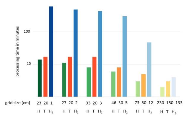
The models proposed by Hu, Tobler, and Hengl were evaluated in eq. (1) on the 1 % training dataset. As noted in eq. (1), the production times of the resulting models were not significantly different between Hu and Tobler, but the Hengl model significantly increased the processing times. The Hu model was adopted because it was more efficient than the Hengl model in terms of time (Fig. 4).
Kriging Structural Analysis
The DEM was produced with 100 % of the training group. A grid size of 23 cm was considered the reference model for both interpolators. When using the Kriging interpolator, it is necessary to set the theoretical semivariogram model of the best fit to the experimental dataset. Fig. 5 was obtained with the ArcGIS Geostatistical Analyst module that optimizes the theoretical function that best represents the behavior of the empirical variable, which is based on the calibration of the plateau coefficients and the range that best conforms to a specific function. The lag size was chosen according to the minimum spacing of the points of the input dataset. Anisotropy was measured between the sample points regarding their distance and direction to determine the spatial correlation. The relation among the sampling points is not invariant as a function of the analysis angle. The amount of data associated with each direction has a different number of samples; in other words, the empirical semivariogram is influenced by the analysis direction.
Heterogeneity exists, noting a greater variation in the correlation of the variable in the west-east direction (XZ plane) and a lower influence over the variogram on the south-north direction (YZ plane) with a slight inclination toward the east.
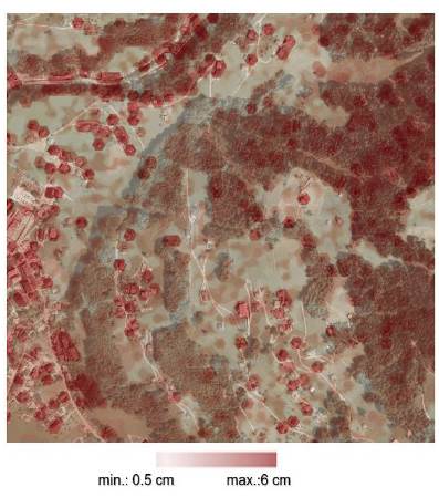
Fig. 6 shows the behavior of the interpolation error where the maximum values appear in the areas with the lowest coverage of ground points; this is justifiable since the interpolation error is associated with the density of the points. These results are in line with those obtained by Liu et al. [33].
IDW Structural Analysis
Contrary to what happens with Kriging, IDW does not make explicit assumptions about the statistical properties of the data, and this algorithm is quite frequent when the data do not fulfill the statistical assumptions. Using cross-validation, the Geostatistical Analyst module optimized the power to which the search distance was raised through the iterative search for the lowest RMSE of prediction. A minimum number of two neighbors and a maximum of eight were used for the weighting. When the structural parameters of the IDW interpolator were fixed, the algorithm was executed.
Interpolation Errors
After producing the DEM, the cross-validation technique was applied to obtain the magnitude of the prediction errors for each training set, as shown in Table 1. Mesa-Mingorance and Ariza-Lopez [34] conducted a critical review of the accuracy assessment of DEMS, arguing that DEMS lack specific guidelines for their evaluation and are considered a challenge for the geospatial community. However, RMSE has been widely used as a quality measurement parameter. Although the RMSE is a widely used measurement, it does not guarantee the absolute quality of the predictions by Zhou et al. [35]. Due to this, this research recurred using MAE, MSE, and E statistics to measure prediction quality. The comparison was carried out using the mean values of the residuals, and this yielded results very close to zero, suggesting that the difference between the RMSE and the standard deviation is not significant, with no presence of systematic errors; however, the overestimation is shown as a generalized tendency for Kriging. The contrary effect is shown by IDW, which mostly underestimated the density elevation and resolution of the evaluated sets.
Table 1 Kriging and IDW prediction errors obtained by cross-validation in centimeters
| Kriging | IDW | |||||||
|---|---|---|---|---|---|---|---|---|
| Density (%) | Points | Average point spacing | Mean | RMSE | Standard error | Mean | RMSE | |
| 100 | 29,385,299 | 22.50 | 0.00 | 5.00 | 2.20 | -0.01 | 5.30 | |
| 75 | 22,038,974 | 25.90 | 0.00 | 5.10 | 2.30 | -0.02 | 6.10 | |
| 50 | 14,692,650 | 31.50 | 0.00 | 5.30 | 2.80 | -0.03 | 6.10 | |
| 25 | 7,346,325 | 43.80 | 0.00 | 5.90 | 3.70 | -0.04 | 7.30 | |
| 10 | 2,938,530 | 67.60 | 0.00 | 7.20 | 5.60 | -0.06 | 9.70 | |
| 1 | 293,853 | 231.00 | -0.15 | 15.50 | 13.90 | 0.19 | 26.90 | |
Source: Own elaboration
Then, the RMSE, MAE, MSE, and E statistics were calculated to evaluate the precision of the elevations estimated concerning the set with original data destined for validation. The results are expressed in Figs. 7, 8, 9, and 10.
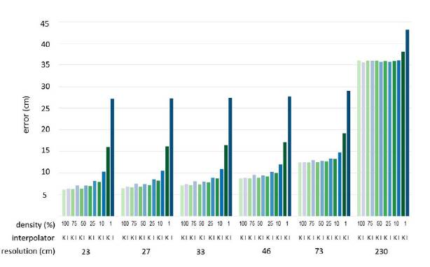
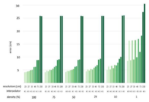
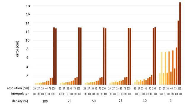
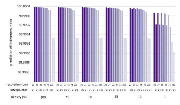
To define the volume and minimum data density, the Paired T Student Test was applied. The results in Tables 2 and 3 indicate that the means of the residuals at different resolutions (except 100 %) are statistically equal to the mean of the training subsets (P-Value > 0.05), which is sufficient to ensure that a higher density setting can be replaced by a lower density set without altering its altimetric quality.
Table 2 Comparative average Kriging residuals
Source: Own elaboration
Table 3 Comparative average IDW residuals
Source: Own elaboration
In the case of Kriging, the grid sizes 23, 27, 33, and 46 cm did not present statistically significant differences between the estimates and the reference DEM, indicating that for these grid sizes, a DEM can be generated using 1 % of the data without altering the sensitivity of the elevation representations. In the case of IDW, the data reduction could only apply from 100 to 75 % with grid sizes of 23, 27, 33, and 46 cm. In their work, Liu et al. [12] were able to reduce 50 % of data the quality of data without altering the DEM using the IDW interpolator.
Morphometric Parameters
The morphometric descriptors slope, curvature, and roughness were calculated for the six grid sizes proposed in each training set, producing 36 surfaces associated with each topographic index. Using the MLR technique and setting the residual errors as the dependent variable and the morphometric parameters as independent, the analysis showed curvature and slope were the variables with the most significant influence on the model. These variables were highly correlated, suggesting that both explain the same thing. They were analyzed individually to leave only one in the model, identifying the one with the highest R2 and the lowest variance. Godone and Garnero [36] studied the influence of morphometric parameters on different interpolators, and their findings pointed to curvature and slope as the main factors that affect interpolation precision. These results are not precisely in line with those found here, given that in their study, they did not use a regression model to detect the correlation between the descriptors.
The linear regression models in Kriging showed that the most influential factor was curvature in all the grid sizes and densities evaluated. For IDW, curvature was also the most influential at 100, 75, and 50 % densities. The roughness indicated an alteration in the prediction in the remaining sets, suggesting that the lack of points produced deficiencies due to the relief complexity.
Multifactor ANOVA was also applied to quantify the residuals' variability by decomposition into slope, curvature, and roughness in each of the associated ranges.
In all cases, the estimated F-Ratio values were to the reference values, right of the reference as shown in Table 4, which indicates that all sources contributed to the representation error of the DEM. After that, multiple range tests were applied to detect which classifications had greater significance within the groups.
Table 4 Analysis of Variance
| Source | Sum of squares | df | Mean square | F-Ratio | Reference | P-Value |
|---|---|---|---|---|---|---|
| Slope | 0.096 | 7 | 0.014 | 3.67 | 2.010 | 0.001 |
| Curvature | 227.814 | 8 | 28.477 | 7656.32 | 1.940 | 0.000 |
| Roughness | 29.906 | 6 | 4.984 | 1340.08 | 2.100 | 0.000 |
| Residual | 12143.8 | 3265011 | 0.004 | |||
| Total (corrected) | 12401.8 | 3265032 |
Source: Own elaboration
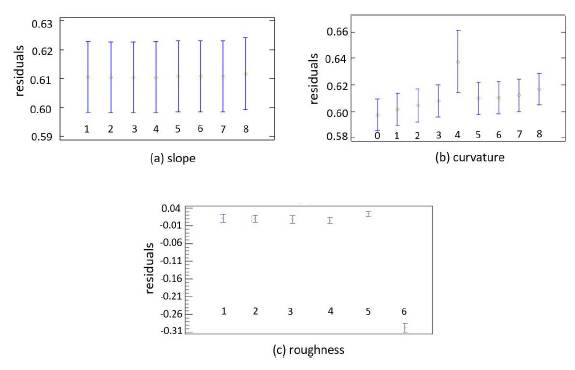
Fig. 11 indicates the mean of the levels in which each factor was grouped. Case (a) represents the influence of the types of slopes over the residuals, detecting no significant differences between any of the slope levels. Case (b) shows the behavior of curvature classification and their associated errors, the plane/plane curvature (Group 4) obtained the highest representation error. Among the rest of the groups, no significant differences were present. Case (c) only presents significance with values associated with high roughness (Group 6).
Spatial Autocorrelation
According to Aguilar et al. [37], when data validation sets are used to evaluate the quality of models and their residues present spatial dependence among themselves, it means that the data validation set must be lower than that currently used, and therefore, a new validation data set must be sought so that it satisfies the following condition: "The spacing between two points must be greater than the maximum distance at which the range is presented "; if this is so, it is said that the residuals of the new set are not autocorrelated having a random spatial configuration; therefore, the error propagation will be independent of location, that is, systematic propagation will not exist within the DEM or its derivative attributes. Supported by this concept, the data validation set was reduced to density levels: 10, 1, 0.5, 0.1, 0.025, and 0.01 %, where only the set of O.O1 % of the original validation information allowed the normality in the residues to be found through the Chi-squared and Shapiro-Wilk tests.
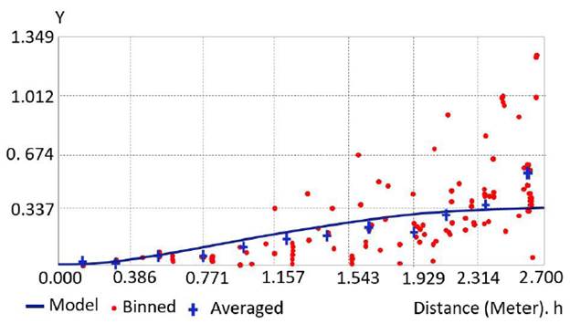
The semivariogram of Fig. 12 was calculated for this last dataset, and a range of 3.99 m was obtained, which compared to the lower spacing between the two checkpoints, which was 7 m, managed to demonstrate thus that the set of residuals is not spatially autocorrelated. Finally, Tables 5 and 6 indicate the maximum data reduction levels without statistically affecting the quality of the DEM and its associated errors.
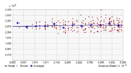
Table 5 Data reduction by Kriging and summary of errors. Units: centimeters
| Set | Grid size | RMSE | E | MAE | MSE | Red. | E | MAE | MSE | MSE |
|---|---|---|---|---|---|---|---|---|---|---|
| 100% | 23 | 6.2 | 100.00 | 4.1 | 0.4 | 99 % | 16.0 | 99.99 | 8.5 | 2.6 |
| 27 | 6.5 | 100.00 | 4.4 | 0.4 | 99 % | 16.2 | 99.99 | 8.7 | 2.6 | |
| 33 | 7.2 | 100.00 | 4.9 | 0.5 | 99 % | 16.4 | 99.99 | 9.0 | 2.7 | |
| 46 | 8.7 | 100.00 | 06.1 | 0.8 | 99 % | 17.1 | 99.99 | 9.9 | 2.9 | |
| 73 | 12.4 | 99.99 | 8.8 | 1.5 | 90 % | 13.3 | 99.99 | 12.0 | 3.7 | |
| 230 | 36.0 | 99.99 | 25.8 | 13.0 | 50 % | 35.9 | 99.99 | 27.4 | 14.5 |
Source: Own elaboration
Table 6 IDW data reduction and summary of errors. Units: centimeters
| Set | Grid size | RMSE | E | MAE | MSE | Red. | E | MAE | MSE | MSE |
|---|---|---|---|---|---|---|---|---|---|---|
| 100% | 23 | 6.4 | 100.00 | 4.3 | 0.4 | 25 % | 7.2 | 100.0 | 4.8 | 0.5 |
| 27 | 6.8 | 100.00 | 4.6 | 0.5 | 25 % | 7.5 | 100.0 | 5.0 | 0.6 | |
| 33 | 7.4 | 100.00 | 5.0 | 0.5 | 25 % | 8.1 | 100.0 | 5.5 | 0.7 | |
| 46 | 8.9 | 100.00 | 6.2 | 0.8 | 25 % | 9.6 | 100.0 | 6.6 | 0.9 | |
| 73 | 2.5 | 99.99 | 8.8 | 1.6 | 50 % | 12.8 | 99.99 | 9.0 | 1.6 | |
| 230 | 35.7 | 99.99 | 25.7 | 12.7 | 75 % | 35.7 | 99.99 | 25.8 | 12.8 |
Source: Own elaboration
Conclusions
This research demonstrated that the reduction capacity of the data volume was affected by factors such as the interpolation algorithm, sampling density, grid size, and terrain curvature. For complex terrain, the LiDAR dataset with an average spacing of 7 m can be reduced to 1 % of its original data density without affecting the quality of the DEM using the Kriging algorithm. This procedure reduces the file size and the processing time for DEM production without compromising the quality of topographic representation.
However, the research results are expected to be improved by analyzing factors such as automatic filtering since it can affect the magnitude of the errors by including erroneous points in the interpolation.

