


 English (pdf)
 Article in xml format
 Article references
 Send this article by e-mail
 Cited by SciELO
  Cited by Google
  Similars in
SciELO
Similars in
SciELO  Similars in Google
 Permalink
The traditional research based on field experiments has a high investment in infrastructure, equipment, labor, and time. Alternatives to conventional studies are the development and application of crop models in agriculture, which show a simplified representation of the processes that occur in a real system, including variables that interact and evolve, showing dynamic and real behavior over time (Thornley, 2011). Crop models allow experimentation, complementing traditional research based on field experiments, and allowing an economical and practical evaluation of the effect of different environmental conditions and several agricultural management alternatives, reducing risk, time, and costs (Ewert, 2008).
Several simulation models have been developed for crops such as cassava (Moreno-Cadena et al., 2020), potato (Fleisher et al., 2017; Saqib and Anjum, 2021), wheat (Asseng, 2013; Iqbal et al., 2014), rice (Li et al., 2015), and corn (Abedinpour et al., 2012; Bassu et al., 2014; Kumudini et al., 2014). Moreover, models are continuously evaluated under different environmental conditions, cultivars, and treatments. These crop models are useful tools for simulations of real crop growth and development processes (Yang et al., 2014). The used models are assumptions that have best survived the unremitting criticism and skepticism that are an integral part of the scientific process of construction and development (Thornley, 2011).
In general, the datasets used to develop a crop model are different from the real inputs in which the model is expected to be used. For a crop simulation model to represent a real process, it must be evaluated considering the differences between crop systems, soils, climate, and management practices; otherwise, the conclusions may be speculative and incorrect (Yang et al., 2014).
The growth dynamics represented by crop models are based on a set of hypotheses, which could result in simulation biases or errors (Yang et al., 2014). Thus, the model performance evaluation is crucial by comparing model estimates to actual values, and this process includes a criteria definition that relies on mathematical measurements of how well the estimates produced by the model simulate the observed values (Ramos et al., 2018). This statistical analysis is considered as the critical method to compare the model outputs with the measured data (Montoya et al., 2016; Reckhow et al., 1990; Willmott et al., 1985; Yang et al., 2000).
The most common methods for assessing the reliability of simulation models are based on the analysis of differences between measured and simulated values, and on regression analysis, also between measured and simulated values (Lin et al., 2014; Willmott, 1982; Yang et al., 2000). However, many authors who research crop modeling use such methods without detailing methodological basis and using terminology and symbols that create confusion. For example, in the analysis of the difference, statistics such as relative error (RE), index of agreement (d), and modeling efficiency (EF) may be useful when comparing the simulation capability of one model with another, but not when comparing what is observed with what is simulated in the same model (Ramos et al., 2018; Yang et al., 2014). Relative error (RE), which relates the error between measured and simulated values, concerning the measured average, represents the relative size of the average difference (Willmott, 1982), indicating whether the magnitude of the root-mean-square error (RMSE) is low, medium or high. However, it has the disadvantage that it can be affected by the magnitude of the values, by outliers, and the number of observations. It may be the case that two groups of data with high and low values, present a similar RMSE. However, having different averages, RE values will also be different (Cao et al., 2012).
Because of its simplicity, regression analysis is often misused to evaluate simulation models. In some cases, the RMSE that measures the average difference between measured and simulated values tends to be used indiscriminately, without considering that it is different from the RMSE obtained in regression analysis (Willmott, 1982). The coefficient of determination (R 2) is a measure of the linear regression adjustment, which, when used in isolation, makes no sense since the goal is to evaluate the crop simulation model, not the regression model obtained.
The magnitude of R 2 does not necessarily reflect whether the simulated data represent well the observed data since it is not consistently related to the accuracy of the prediction (Willmott, 1982). This is because an R 2 can be obtained close to 1.0 but below or above the 1:1 line, tending to simulate high values or underestimates the observed values, respectively.
Many statistical indices are frequently used in model evaluation, and this paper aimed to compare and improve the understanding and interpretation of these conventional statistical indices in a case study.
MATERIALS AND METHODS
The performance of nine statistical indices was computed to evaluate the simulations of actual observations and simulations of total dry weight (kg ha-1) obtained in a diploid potato field experiment conducted in Medellín, Colombia. This data set were taken from Saldaña-Villota and Cotes-Torres (2020). Besides, from the actual observed data, six data sets were generated with arbitrary deviations appropriately imposed to illustrate the behavior of the statistical indices under evaluation. (Table 1). In case 1, the first half of the simulations is overestimated, and the second half is underestimated in the same amount (200 kg ha-1). In case 2, the first half of the simulations is overestimated 1.5 times, and the second half of the simulations is underestimated 0.5 times. In case 3, all simulations are overestimated in 100 kg ha-1. In case 4, all simulations are overestimated 2.5 times. In case 5, most of the simulations are overestimated in different proportions, and an outlier 3.4 times larger than its corresponding observation is presented. Finally, in case 6, all simulations are overestimated in different proportions, and they do not have any relationship with the observations.
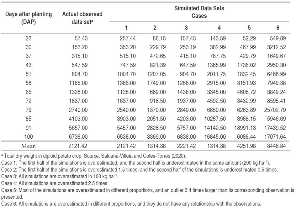
The indices are expected to inform the researcher of the accuracy of any model in simulating the observations. The statistical indices are expected to allow decisions to be made regarding the acceptance or rejection of the models. In this study, with the modifications applied to generate the six cases, the statistical indices must accept cases 1 and 3 and reject the other cases without ambiguity.
Many statistical indices are commonly used in model evaluation, and they have been classified depending on their mathematical formulation. In this study, nine indexes were evaluated and classified into two categories. The first one corresponds to the 'test statistics', and the second one corresponds to measures of accuracy and precision called 'deviation statistics' (Ali and Abustan, 2014; Willmott et al., 1985; Yang et al., 2014).
Test statistics
Linear regression and coefficient of determination (R 2) are used to explain how well the simulations (y) represent the observations (x) (Kobayashi and Salam, 2000; Moriasi et al., 2007; Willmott, 1982). The linear model follows Equation 1.

where α is the regression intercept, β is the slope, and ε represents the random error.
The R 2 assesses the goodness of fit of the linear model by measuring the proportion of variation in y, which is accounted for by the linear model. R 2=1.0 indicates a perfect fit of Equation 1, and R 2=0 means there is no linear relationship.
However, many researchers have reported the limitation of R 2 in the appropriate evaluation of the models, remarking that R 2 estimates the linear relationship between two variables, and it is no sensitive to additive and proportional differences between model estimates and measured data (Kobayashi and Salam, 2000; McCuen and Snyder, 1975; Willmott, 1981). The authors also indicate that the relationship may be non-linear, which would be an additional problem.
Deviation statistics
Some deviation statistics correspond to measures developed to test the deviation directly (deviation = y-x)and surpass the limitation of correlation-based statistics (Yang et al., 2014). The Mean Error (E) (Equation 2) indicates whether the model simulations (y) overestimate or underestimate the observations (x). When E>0 means that the model is overestimating, while E<0 means that model underestimates the measured data. E has a drawback: the positive and negative errors can negate each other, and large positive and negative deviations can still obtain E-0 (Addiscott and Whitmore, 1987; Yang et al., 2000).

where i-1,2,...,n .
Due to E disadvantage, some measures based on the sum of squares were developed (Yang et al., 2014). The root mean square error (RMSE) (Equation 3) has the same unit of deviation y-x, and it is frequently used in both model calibration and validation process (Hoogenboom et al., 2019; Hunt and Parsons, 2011)

The relative root mean square error (rRMSE) (Equation 4) is a relative measure used for comparisons of different variables or models. indicating whether the magnitude of the root-mean-square error (RMSE) is low, medium, or high (Priesack et al., 2006).

Nash-Sutcliffe modeling efficiency coefficient (EF) (Equation 5) (Nash and Sutcliffe, 1970). This index is a dimensionless measure (-∞ to 1.0). A perfect fit between simulations and observations produces an EF-1.0.
Any value between 0 and 1.0 is obtained for any realistic simulation. EF<0 is obtained if the simulated values are worse than merely using the observed mean to replace the simulated y i.

Another index that is commonly used in crop model evaluation is the index of agreement (d) (Equation 6) a dimensionless measure (0 to 1.0) proposed by Willmott (1982). This index has been recommended by researchers in modeling to carry out comparisons between simulated values and measured data (Krause et al., 2005; Moriasi et al., 2007).

EF and d are more sensitive to larger deviations than smaller deviations. The main disadvantage of both statistics is the fact that the differences between model estimates and observations are calculated as squares values; thus, these sums of squares-based statistics are very sensitive to outliers or larger deviations due to the squaring of the deviation term (Krause et al., 2005; Legates and McCabe Jr, 1999; Willmott et al., 2012).
To overcome the difficulty of the statistics based on the sum of squares that are inflated by the squaring deviation term, statistics based on the sum of absolute values were proposed (Krause et al., 2005; Willmott et al., 2012). The modified efficiency coefficient (EF 1) (Equation 7) replaces the sum of squares term with the sum of absolute values of y-x . EF 1 is less sensitive to outliers, and it takes also values between -∞ and 1.0 (Legates and McCabe Jr, 1999).

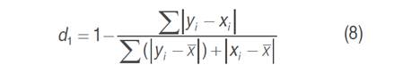
Willmott et al. (1985) proposed the modified index of agreement (d 1) (Equation. 8), to avoid the critical effect of outliers in the sum of squares used on d. The author remarks that d 1 yields 1.0 more slowly than d. d and d 1 show relative high values even if a substantial deviation is evident, and to overcome this issue, Willmott et al. (2012) proposed a refined index of agreement (d 1') (Equation 9), which is ranged -1.0 to 1.0. When , d1'=0.5, the sum of the magnitude of the errors is half of the sum of the perfect-simulated-deviation and observed-deviation magnitude.

The calculation of the statistics indices to evaluate the six simulated data sets, and figures were made with R statistical software (R Core Team, 2020).
RESULTS AND DISCUSSION
This study shows a comparison of nine statistical indexes used during model evaluation. The actual data of the total dry weight measured in a diploid potato field experiment and the six simulated data set are shown in Figure 1 to facilitate the visualization of the data and their analyzes.
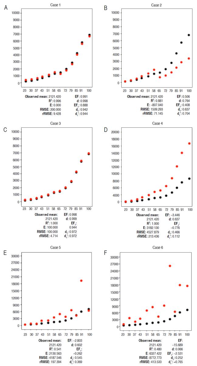
Figure 1 Comparison between real observations and six simulated data set of total dry weight in diploid potato crop (kg ha-1) over time (days after planting). Black circles correspond to the real observations, and red ones correspond to the simulated counterpart.
Coefficient of determination (R 2 )
In the simulated data cases 1, 2, 3, and 4 (Figure 1A-D), different scenarios were presented in which the actual observations are overestimated or underestimated. The simulations preserved the trend of the measurements, which is the reason why the R 2 was high. Although simulations considerably overestimated the measurements in case 4, the fact that the simulated data follow the trend of the observations even if they are overestimated or underestimated, the R 2 will be close to 1.0. Consequently, this index is not adequate to evaluate the quality of the simulations in growth variables in crop models. The coefficient of determination was lower in cases 5, and 6 (Figures 1E and F), indicating that the simulated data did not follow the observed data trend.
Mean error (E)
E indicates whether the model overestimates or underestimates the measurements. This index presented difficulty to indicate what happened in case 1, in which half of the simulations were overestimated, and half were underestimated in the same proportion. In this case,E-0, and this value gives no indication of over or underestimation. In case 2, E indicates that the simulated data underestimate the total dry weight by 807,040 kg ha-1. In the remaining cases, E>0, indicating that the simulations overestimate the measurements. According to E, case 6 was the one that registered the maximum overestimation, exceeding 6000 kg ha-1.
Root mean squared error (RMSE) and the relative-RMSE (rRMSE)
The RMSE indicates how deviated the simulated mean is from the observed mean. This index does not indicate whether there are overestimates or underestimates. Nevertheless, if the RMSE is close to zero or less than the amount assigned by the researcher according to the expertise in the crop studied, the model performs better in predicting the measured data. If the researcher is not an expert about the range of values that a growth variable can reach, the RMSE should be evaluated together with rRMSE, which indicates the deviation of the simulations from the general mean of the observations in percentage terms. In this sense, according to the characteristics of these two indices, unquestionably cases 1 and 3 had the best performances when simulating the observations, where the deviation from the mean was 200 and 100 kg ha-1, corresponding to 9.428 and 4.714%, respectively.
Regarding case 2, where the simulations underestimated the total dry weight from 65 DAP, the RMSE was affected, recording a value of 1509.293 kg ha-1, meaning a deviation higher than 70% (rRMSE). In case 4, although as mentioned, the simulations overestimated the observations even though they followed their trend. This overestimation significantly influenced the RMSE, which registered a value of 4527.879 kg ha-1, equivalent to a deviation of more than 200% concerning the general mean of the observations (2121.42 kg ha-1). Case 5 exemplifies the effect that outliers have on statistical indices. At 91 DAP, a very high datum was recorded in the simulations compared to the other simulations and, of course, to the observations. Together with the other predicted data, this outlier generated RMSE-4187.516 kg ha-1, and rRMSE-197.394%. If the researcher, after exploring different explanations for this extreme data, decides not to consider the outlier, the RMSE would be equal to 2320 kg ha-1 and the rRMSE-10939%, indicating that in the same way, the model does not predict the observations in an acceptable way and these are overestimated at 2130 kg ha-1 (keeping the outlier) and at 547.96 kg ha-1 (eliminating the outlier). Finally, the RMSE and rRMSE obtained in case 6 are definitive to consider that the simulations are unacceptable. Although the graphical representation (Figure 1F) is a clear indication of the low quality of the predictions, an RMSE-8772.773 kg ha-1 and an rRMSE higher than 400% are enough to rule out the model. Besides, this data set had outliers, but in general, the simulated data had no relationship with the observations.
Nash-Sutcliffe coefficient (EF) and the modified Nash-Sutcliffe coefficient (EF1)
The analysis of the following indices that are dimensionless, such as the Nash-Sutcliffe coefficient (EF) and the modified Nash-Sutcliffe coefficient (EF 1), confirm that simulations in cases 1 and 3 are close to perfection with values very close to 1.0 (EF-0.991 and 0.998; EF 1-0.888 and 0.972, respectivelty).
According to Nash and Sutcliffe (1970), EF and EF 1 values between 0 and 1 are expected in any modeling scenario. However, in case 2, for instance, EF and EF 1 reached values of 0.506 and 0.408, which are values higher than zero, but by themselves, they are not clear with the reality of the simulation quality. Nonetheless, values less than zero in these two indices are indicators of wrong predictions; thus, cases 2, 5, and 6 achieved values <0, confirming what E, RMSE, and rRMSE had indicated. Also, the more negative values suggest that the simulated data were worse. The clearest example is case 6, which reached -15.689 in EF, but EF 1 was -2.531. EF reached higher values (both positive and negative) because when considering sums in terms of the sum of squares in its formulation, it is more affected by outliers. EF 1 is calculated considering the sum in terms of absolute values, that means less sensitivity to extreme data.
Index of agreement (d), modified index of agreement (d 1 ), and revised index of agreement (d 1 ')
Finally, from the group of indices d, d 1, and d 1', the best simulations reach values close to 1.0 (Cases 1 and 3). In the same way as EF and EF 1, the statistics of group d must be estimated in association with other indices to make better inferences about the accuracy of the simulation. In case 2, d=0.764, and if this value is analyzed by itself, it would suggest that the model is adequate, but d1 is stricter than d, and its value is clearer suggesting that the simulations are not adequate (d 1=0.637). d and d 1 in cases 5 and 6 were less than 0.75, suggesting that these models are not suitable for simulating the measured data set. Case 6 was the only one that reached a negative d 1' value (-0.765), again indicating that the simulations, in this case, are not adequate when predicting the measurements.
General performance of the statistical indices in evaluating the quality of the simulations of a model
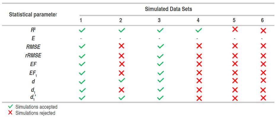
Summarizing the previous results (Table 2), the RMSE, rRMSE, EF, EF 1, and d 1 are the best indices for evaluating the quality of simulations because, they accepted the simulations in cases 1 and 3, and rejected the other cases, which was expected in this study when comparing the behavior of the statistical indices. However, given the simplicity in the interpretation of RMSE and rRMSE, they are preferred over dimensionless statistics.
Table 2 Acceptance or rejection of the simulations defined by different statistical indices for each data set.
Statistical analysis is a crucial procedure during model calibration and evaluation, and there are many statistical methods useful to support crop model researchers. It is unquestionably that R 2 is not a suitable parameter for model evaluation because it is not sensitive to additive (regression intercept) and proportional differences (regression slope) (Willmott et al., 2012; Yang et al., 2013). The linear regression should be employed to evaluate the simulated outputs with the observed inputs when the time series data follow the assumptions of independence, normality, and homoscedasticity in the error term (Yang et al., 2014). The error term does not follow these assumptions in the deviation statistics because they are not hypothesis tests (Willmott et al., 1985).
The mean error (E) is a good statistical parameter to quickly determine if the model under or overestimates the observations. Unfortunately, it does not offer clarity on the quality of the simulations. Nevertheless, RMSE and rRMSE are very suitable for model evaluation because they provide the researcher with a useful decision-making guide. It is important to highlight the advantages that the RMSE and the rRMSE offer, which together offer a better idea of how deviated the simulations are in the same unit of the variable and percentage terms.
If only the group index of agreement is considered during the evaluation of a model, it is possible to make bad decisions or assume that the model predicts the measured data with quality when in reality, the predictions are not adequate. d can quickly reach 1.0 without considering significant discrepancies between simulations and observations because the sum of squares-based deviations easily inflates d. A researcher could consider case 2 a suitable model to simulate the observations according to d and d 1' values, even when d 1' seems to be stricter than d in mathematical terms. d 1 and EF showed well behaviors, and they have a sharp meaning and interpretation when values tend to zero. Yang et al. (2014) suggested for plant growth variables simulations EF>0 and d, d 1, and d 1' as minimum values for dry weight of leaves, stems, yield, tubers, total in the case of the potato crop.
Both modeling efficiency coefficients (EF and EF 1) and indices of agreement (d, d 1, and d 1') are widely used in modeling evaluation. Although d and EF are sensitive to the sum of squares and, in consequence, they achieve higher values even with not accurate simulations. The researcher should use these dimensionless indices carefully. Alternatively, use RMSE and rRMSE as good guides to evaluate the quality of the models.
CONCLUSION
The RMSE and the rRMSE offer a better idea of how deviated the simulations are in the same unit of the variable and percentage terms; for this reason, these indices are the most appropriate to reflect the quality of the simulations of a model. This pair of indices was the only one that unquestionably established that cases 1 and 3 are almost perfect with deviations less than 200 kg ha-1, which is less than 10% concerning the mean of the observations. RMSE and rRMSE leave no doubt that cases 2, 4, 5, and 6 correspond to models that reflect very poorly or do not reflect the observations.

