


 Inglês (pdf)
 Artigo em XML
 Referências do artigo
 Enviar este artigo por email
 Citado por SciELO
  Citado por Google
  Similares em
SciELO
Similares em
SciELO  Similares em Google
 Permalink
Introduction
The current lack of understanding of the causal agent of LW leads to uncertainty about the influence of various factors on the dynamics of the disease, which makes it difficult to develop a management plan. In this context, it has been necessary to largely resort to plantations history and basic management practices such as the reduction of the inoculum starting from the early elimination of diseased palms, which implies a strict follow-up, to the appearance of cases through weekly phytosanitary censuses (Cenipalma, 2019). Thus, those who have to deal with the disease have extensive records of historical data. However, there are few methodological tools that allow converting these data into information and, from there, into knowledge about the behavior of the disease on a time scale.
An epidemic in a crop can be regarded as a change in the incidence of the disease in a host population over time and space. The characterization of the progression of those changes over time can provide valuable epidemiological insights. This characterization is important to understand how diseases develop in plant populations and how management measures affect epidemics (Campbell & Madden, 1990; Van der Plank, 1963). The graphical representation of the incidence of a disease (y) versus time (t) is known as disease progression or development curve. For many purposes, this is the main description of an epidemic and focuses on the interactions occurring among the host, the pathogen, and the biological and physical environment in the development of the disease whose main objective is to understand the complex interactions occurring. This information can be used, for example, to predict the incidence of the disease at a given time, quantify the effects of management strategies on epidemics, or, ultimately, to develop a theoretical basis for determining whether an epidemic might occur, and, if it does, to identify the factors affecting both the disease development rate (r) and its final incidence (y 1 ) (Madden, et al., 2007; Xu, 2006).
In principle, plant disease epidemics can be classified into two basic types, monocyclic and polycyclic, depending on the source of the inoculum that comes into contact with the host over the course of the disease and the number of infection cycles per crop cycle (Madden, et al., 2007). Therefore, the classification of an epidemic as monocyclic or polycyclic depends on the type of behavior over time as measured by the level of adjustment of the different growth models to the values observed in the field. Thus, a monocyclic epidemic can be described quite well using a monomolecular model while a polycyclic epidemic can be described with a logistic or Gompertz model (Arneson, 2001). Epidemiological processes are characterized by using growth models with varying degrees of complexity. The selection of an appropriate model allows the characterization of an entire epidemic with few parameters. It is, therefore, relatively easy to compare epidemics and assess the effects of biological and environmental factors, as well as the possible managements for implementing more effective, efficient, and sustainable strategies in integrated disease management (Forrest, 2007; Madden, 1986). The resulting disease development curves are graphical representations of the development dynamics of the epidemics and their parameters can be fitted to the obtained data using any standard statistical package (Van Maanen & Xu, 2003; Neher, et al., 1997). In this line, multiple fully functional applications have been developed in different programming languages such as Java, with the EpiModel software (Nutter & Parker, 1997) and Excel spreadsheets (Bowen, 2015), and R packages such as epiphy (Gigot, 2018) and epifitter (Alves & Del Ponte, 2021).
Most of the mathematical models used for determining disease progression curves can be estimated using only two parameters such as y 0 (initial disease or constant of integration) and r (rate of disease development). Using these two, two or more epidemics can be compared and a considerable understanding of disease dynamics is achieved. However, not all epidemics can be described by two-parameter models (Madden, et al., 2007). The values observed over time in the development of a disease do not often fit any specific model, which most probably reflects the fact that the biological basis of the models is only a simple approximation to a much more complex pathosystem and, consequently, the model lacks the necessary flexibility to be adapted to various aspects of the development of the disease (Park & Lim, 1985). The classical growth-curve models for epidemics analysis include several implicit assumptions, which may lead to misinterpretations about the progression of the disease if they are not considered (Neher & Campbell, 1992). Many of those models, such as the monomolecular, logistic, and Gompertz, assume a constant host area that becomes diseased by the end of the epidemic implying a maximum disease incidence of 100%. Consequently, the models used to describe epidemics assume an asymptote or a maximum disease incidence (Kmax) equal to 1 (Campbell & Madden, 1990; Seem, 1988). However, this assumption is not valid for many diseases and the mathematical description of the epidemic is thus inaccurate, imprecise, and inappropriate. Besides, in some epidemics, such as rusts, powdery mildews, and viral diseases caused by obligate parasites, it is only possible to visualize a maximum disease intensity between 25 and 40%, far below the expected 100% (Jeger, 1982; Campbell & Madden, 1990; Gilligan, 1990; Kranz, 2003; Madden, et al., 2007). This has resulted in the ongoing use of growth models for epidemiological analysis that do not consider the maximum disease intensity. Consequently, important parameters, such as the growth or disease development rate, are not properly estimated, or, simply, a given disease is analyzed in a model with different behavior.
Several researchers have reported this type of error in the description of epidemics. For example, Turner, et al. (1969), Kiyosawa (1972), and Analytis (1973, 1979) agreed that the value of the asymptote or the Kmax could affect the calculation of r in generalized Logistic models in the description of epidemics. Kushalappa & Ludwing (1982) indicate that empirically determining the value of the asymptote (Kmax) greatly improves the goodness of fit of disease development models. Park & Lim (1985) mathematically illustrate how disease development rates (r) are underestimated when calculated with traditional models under the assumption that the maximum disease incidence is 1 (Kmax = 1) when really the maximum incidence is below this value (Kmax <1).Neher & Campbell (1992) quantified the magnitude of underestimation in r when values above a real incidence are assumed in models such as the monomolecular, logistic, and Gompertz. Since Kmax affects rates of disease development, Neher & Campbell (1992) suggested for Kmax <1 shape parameters m with the values 0, 1, and 2 for the monomolecular, Gompertz and logistic functions, respectively, to use weighted mean absolute rates p = r K/(2m + 2) with K= Kmax and the rate disease progress r calculated by the function used to fit the curve. This approach introduces the shape parameter m as a measurement term and descriptor. Parameter K can be dropped from the equation (if different with the same m) and then rK could be calculated as an overall (mean) measure of the absolute rate of disease development (Neher & Campbell, 1992). Although this approach manages to correct the underestimation of parameters such as the rate (r) of development of the disease, it fails to improve the classification of the model that best fits, which still leads to generating erroneous or biased interpretations of pathosystems with monocyclic or polycyclic behaviors completely different from the real one. The objective of the following study is to demonstrate the error committed in the classification of the model that best fits the data when Kmax is lower based on the temporal analysis of three epidemics caused by lethal wilt (LW) in oil palm (Elaeis guineensis Jacq.) plantations.
Methodology
Plot selection
We obtained the historical disease monitoring records for three plots sowed with susceptible cultivars of E. guineensis between January 2015 and December 2017 (36 months) at the Luker Agrícola (4°35'N, 72°49'W, 198 m. a.s.l.) and Palmar de Oriente plantations (4°29'N, 72°50'W, 195 m. a.s.l.) located in the municipality of Villanueva (Casanare), Colombia, an area with a high incidence of the disease. The three plots we selected satisfied the following characteristics (listed from highest to lowest importance): (i) final incidence with the highest record (y1); (ii) known initial incidence (y0), and (iii) records with the longest follow-up time (t). All historical disease-monitoring records were done palm by palm by personnel trained in the detection of plants with initial symptoms of the disease at 30-day intervals. The total population of plants evaluated from plots 1, 2, and 3 corresponded to 1,315 (8.5 ha), 2,842 (17.8 ha), and 2,835 (17.7 ha), respectively.
Models used when Kmax is a parameter
Given that the monomolecular, logistic, and Gompertz models generally assume that the maximum disease incidence is 1, we modified the mathematical equations of the traditional models in terms of proportion to the differential, nonlinear, and linearized versions in which the maximum disease incidence was a parameter (Table 1).
Table 1 Differential, nonlinear, and linearized equations of the models used to analyze the disease progression data when the maximum disease incidence (Kmax) is a parameter

Source: Campbell, 1998
K: Kmax: maximum disease incidence (y) or asymptote of the disease progression curve; Y: disease in proportion at the time of observation; y0: disease in proportion at the first observation; r*: disease growth rate of a specific model; t: considered time interval
Assessment of goodness of fit of the models
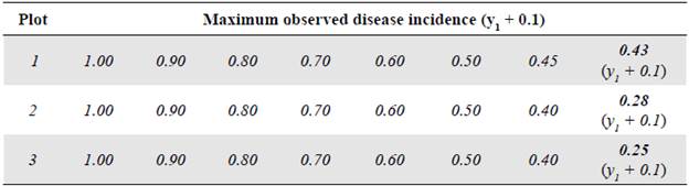
We assessed the goodness of fit of the monomolecular, logistic, and Gompertz models at different final incidences including the maximum observed (y 1 + 0.1), which were 0.43, 0.28, and 0.25, respectively (Table 2). Then, we subjected the data to linear regression analysis, analysis of variance, and distribution of residuals using R v1.1.463 (R Core Team, 2018) and the statistical package 'nlme v3.1-144 (Pinheiro, et al., 2004). We calculated the F-test on the estimated parameters as the ratio between each of them and the asymptotic standard error to determine whether the parameters contributed to fit the model. Higher F-values are associated with higher contributions of the estimated parameters to fit the model (Hosmer & Lemeshow, 2000). The asymptotic standard error is used to assess the goodness of fit of the models to the real points of the epidemic using the least-squares regression associated with the coefficients estimated by each model. It is accepted that small standard errors indicate more accurate estimates (McCullagh & Nelder, 1992).
Comparison of the goodness of fit of the models
We used the statistical package ' AICcmodavg v2.2-2 (Mazerolle, 2019) to compare the goodness of fit of the models for each Kmax while the relative goodness of fit of the three models was determined from the estimated coefficients of determination (R2) and the implementation of the Akaike (AIC) and Bayesian (BIC) information criteria.
The R2 of the linear regression analyses determines the ability of the model to replicate the results and the proportion of variation of the results that the model can explain. A coefficient value closer to 1 means less variation in the estimate. The AIC uses a relative value between the goodness of fit of the model and its complexity calculated by the formula AIC = -2 log(L(θ|y)) + 2K, where log(L(θ|y)) is the numerical value of the log-likelihood function at its maximum point and K is the number of estimated parameters in the function. The BIC applies a higher penalty for the number of parameters in the model calculated by the formula BIC = -2 log(L(θ|y)) +K log n; as in the previous formula, log(L(θ|y) is the numerical value of the log-likelihood function at its maximum point, Kis the number of estimated parameters in the function, and n is the number of parameters in the model. The farther the AIC and BIC values are from zero, the higher the goodness of fit of the model to the observed values (Burnham & Anderson, 2002).
Results and discussion
After 36 months of observations in the three epidemics evaluated, 15, 22, and 18 plants died on average per month, respectively, for a total of 2,001 plants, i.e., 29% of the 6,992 plants evaluated. We assessed all models based on their goodness of fit measured by linear regression tests, analysis of variance, and 95% confidence intervals. Table 3 shows the F-test values of the least-squares method for the analysis of variance, the coefficient estimates, the asymptotic standard error, and the 95% confidence interval for the coefficients of the three models estimated at different maximum incidences of LW in the three analyzed epidemics, respectively (Table S1, S2, and S3, https://www.raccef.yn.co/index.php/raccefyn/article/view/1571/3188).
The F-test values indicated that the estimated parameters contributed significantly to the fit of the disease progression curves in the three epidemics, regardless of the maximum disease incidence. We also found that the estimates calculated by the three models contributed significantly to the fit of the coefficients y 0 and r by confirming that the 95% confidence intervals did not contain a value equal to zero.
A more detailed analysis of the F-test and the asymptotic standard error per plot revealed variations between the models as the maximum incidence parameter was adjusted to a real value of the disease. In general, the monomolecular model showed higher F-test values and lower asymptotic standard errors when we assessed maximum asymptotes of 1.0, 0.9, 0.8, 0.7, 0.6, and 0.5 in the epidemics. However, there were evident changes as the maximum incidence parameter (Kmax) was adjusted to the real observed value changing from the monomolecular to the Gompertz model in the analyzed epidemics with maximum asymptotes of 0.45 and 0.43, 0.40 and 0.28, and 0.25 (Table 3) corresponding to plots 1, 2, and 3, respectively.
Table 3 Linear regression analysis of the three growth models assessed at different asymptotes or maximum disease incidence (Kmax) of the records corresponding to plots 1, 2 and 3

Values in bold indicate coefficients with the highest contribution to the model fit according to the standard asymptotic error test. ** Level of significance of 1%; 1y0: disease in proportion in the first observation; 2r*: disease growth rate of a specific model
Figures 1, 2, and 3 represent the variations when the parameter Kmax changed from a theoretical value (Kmax = 1) to a real value and its effect on the estimates of the LW development rate. The R2 and the AIC and BIC applied to assess the relative goodness of fit of the model to the data observed showed the same trend evident in the F-test, the asymptotic standard error, and the graphic representations of the goodness of fit of the models (Figure 4).
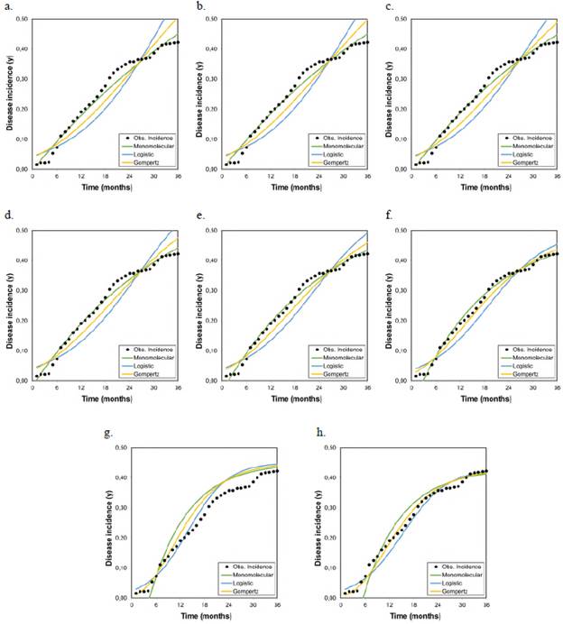
Figure 1 Graphical representation of the goodness of fit of the models to the disease progression curves at different asymptotes or maximum disease incidences (Kmax) corresponding to the records collected from plot 1 r M , r L , and r G represent the growth or disease development rates in the monomolecular, logistic, and Gompertz models, respectively.
As the Kmax parameter approached the theoretical maximum incidence (Kmax = 1), the model that best fitted the observed values in the three analyzed epidemics was the monomolecular. However, its goodness of fit in each of the tests did not faithfully represent the behavior of the disease when the actual maximum incidence was much lower than 1. When the Kmax was assumed as the real one, i.e., 0.43, 0.28, and 0.25 for epidemics 1, 2, and 3, respectively, the goodness of fit measured by the R2 from the linear regression analyses and the AIC and BIC showed that the model that best fitted the observed values was the Gompertz.
These results demonstrate that the monomolecular model has high sensitivity when assuming a theoretical asymptote equal to 1 (Kmax = 1), which was further supported by the values obtained in the R2, AIC, and BIC analyses. When the asymptote was below 0.50, the goodness of fit gradually decreased and other models with better fits acquire major importance as is the case of the Gompertz model given that with the maximum observed incidences (0.43, 0.28, and 0.25 for plots 1, 2, and 3, respectively), the LW development curves were fitted to the development curves observed in the three epidemics (Figures 1, 2, and 3). It was clear from these Figures that below 0.50, the best settings of LW development rate were achieved when the models were fitted to the maximum disease incidences with low values. Consequently, the underestimation of highly relevant epidemiological parameters, such as the rate (r) of disease development, is extremely likely not only in sensitive models such as the monomolecular one but also in the logistic and Gompertz models when the maximum disease incidence is assumed to be higher than the real value.
Park & Lim (1985) initially observed that assuming an asymptote equal to 1 in logistic functions can lead not only to underestimate the rate (r) of disease development but also to incorrectly classify its values when fitting a data set with real asymptotes below 1 differing from each other. Neher & Campbell (1992) found that the greatest underestimation of the rate (r) of disease development occurred most notably when they used the monomolecular model and the r was higher when Kmax diminished considerably, regardless of the rate of disease development or growth rate, which agrees with our results. Furthermore, these authors concluded that the extent of disease development rate underestimation depended on the model, the disease growth rate itself, and the proximity of the real value of Kmax to 1 because underestimations were more pronounced with lower real maximum incidence values, higher disease growth rates, and prolonged epidemics.

Figure 2 Graphical representation of the goodness of fit of the models to the disease progression curves at different asymptotes or maximum disease incidences (Kmax) corresponding to the records collected from plot 2 r M , r L , and r G represent the growth or disease development rates in the monomolecular, logistic, and Gompertz models, respectively.

Figure 3 Graphical representation of the goodness of fit of the models to the disease progression curves at different asymptotes or maximum disease incidences (Kmax) corresponding to the records collected from plot 3 r M , r L , and r G represent the growth or disease development rates in the monomolecular, logistic, and Gompertz models, respectively.
Recently, López-Vásquez, et al. (2021) conducted a study to identify suitable tools for the epidemiological analysis of the LW pathosystem and found that the exponential, monomolecular, logistic, Gompertz, and Richards models using a Kmax = 1 did not meet the assumptions of normality and constant variance, which resulted in a poor fit of the models to the observed values, both in linear and nonlinear models, thereby considering the area under the disease progression curve (AUDPC) as a descriptive alternative for this disease. The variation of the models best fitted to the observed data in the three epidemics we evaluated was influenced by the change in the maximum incidence. This variation in the goodness of fit associated with the maximum incidences was more evident in the monomolecular model than in the logistics and Gompertz models as the Kmax parameter approached the absolute value of 1. However, this trend changed when it was adjusted to the maximum real disease incidence while the Gompertz and logistic models had a better fit of the data to the observed values in the three epidemics.
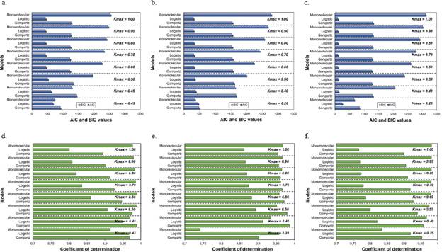
Figure 4 Goodness of fit measured by the Akaike (AIC) and Bayesian (BIC) information criteria (A, B, and C) and the coefficients of determination (R2) of the linear regression analyses (D, E, and F) for each of the three growth models analyzed at different asymptotes or maximum disease incidences (Kmax). A and D. Plot 1; B and E. Plot 2; C and F. Plot 3
Our results demonstrated the sensitivity of the monomolecular model when the maximum disease incidence was assumed as higher than the real value. Besides, this model was the only one that tended to an increase in the goodness of fit when the maximum disease incidence values were approaching 1, as opposed to the logistic and Gompertz models that had stable values regardless of the increase in the maximum incidence. All epidemiological procedures used in this study showed that assuming 100% of the maximum disease incidence (Kmax = 1) when the final disease incidence was below this value had a significant effect on the epidemiological analysis producing inaccuracies not only by underestimating the rate of disease development but also in the selection of the best-fit model, which consequently led to errors in the mathematical description of the epidemic.
Our results also confirmed the empirical estimations made by Analytis (1973) and Park & Lim (1985) to conclude that calculations with Kmax = 1 affected the value of r in the case of an actual asymptote of disease intensity below 100%. Hence, K = 100% as disease intensity should not be indiscriminately used in equations to compute rates. In fact, Madden, et al. (2007) raised the possibility of including Kmax as an additional parameter in the characterization of the dynamics of the disease given the difficulty of the objective description of epidemics with only two parameters (y0: initial disease or constant of integration and r rate of disease development). Currently, R packages such as epifitter (Alves & Del Ponte, 2021) have a function that fits modifications of the two-parameter models to account for this additional parameter as the maximum asymptote.
On the other hand, if the epidemic had been characterized with the type of model that best fitted the data when Kmax = 1, the LW epidemic would have been classified as having a monocyclic behavior given that the best settings were obtained with the monomolecular model. However, when we adjusted the Kmax to the actual Kmax < 1, the LW epidemic changed from a monocyclic to a polycyclic behavior because the best-adjusted models were those of the Gompertz type. These types of results have epidemiological implications in result analyses, as well as technical implications in the strategic management of the disease because a significant part of the comprehensive management strategy of the disease is based on the type of behavior of the epidemic. It is important to note that given that WL is currently considered an official control disease in Colombia (Resolution 004170; ICA, 2014), all the plots we selected were continuously subjected to phytosanitary measures for foci management and containment. This kind of anthropogenic event explains to a certain extent why this epidemic had such low final incidences in a given time period. Additionally, we should keep in mind that time (t) is a continuous parameter and, therefore, a 36-month-period cannot be considered the total length of an epidemic in a crop such as oil palm with an eventual economic life span of up to 25 years. This could be different in a semiannual crop that can be harvested in less than 12 months. Therefore, it is possible that a longer time (more than 36 months) of evaluation may result in additional increases in disease incidence given the availability of healthy tissue, which could reach 100 % if no management practices are performed.
Conclusions
One of the main purposes of epidemiological analyses using models is to achieve a better understanding of how diseases develop in plant populations over time and how other factors influence their development. When selecting an appropriate model, one must have the ability to understand and explain the factors associated with the estimation of the parameters that describe the epidemic. However, the models often lack the necessary flexibility to adapt to the various changes occurring during the development of a disease. In this sense, the goodness of fit of a model depends on the increase in the number of estimated parameters and, consequently, on the flexibility of the selected model.
Although the true asymptote for the development of any disease is a function of the amount of susceptible tissue available, we should be aware of the risk of assuming a theoretical value of the maximum disease incidence in the host in a generalized and arbitrary manner. There are many epidemics with a maximum incidence below 100% due to unfavorable environments, insufficient populations of insect vectors or propagules, levels of host resistance, disease reduction practices focused on the early elimination of diseased plants, or other unspecified physical or biological factors.
Our results demonstrate the importance of including Kmax in the description of the temporal behavior of an epidemic. The consequences of using incorrect values reflect not only in the erroneous estimation of parameters, such as y 0 and r but also in the risk of incorrectly interpreting the temporal behavior of the epidemic because of a false fit of the selected model. Assuming the parameter Kmax as unique and absolute may lead to inaccuracies in the type of epidemiological analysis and, consequently, to a biased description of reality.

