L.V. Eppelbaum¹, I.M. Kutasov¹ and G. Barak¹

¹Dept. of Geophysics and Planetary Sciences, Raymond and Beverly Sackler Faculty of Exact Sciences, Tel Aviv University, Ramat Aviv 69978, Tel Aviv, Israel
Corresponding Author: L.V. Eppelbaum, e-mail: levap@post.tau.ac.il

ABSTRACT

Understanding the climate change processes requires application of special methodologies for revealing a ground surface temperature history (GSTH). It was proved by different authors that the GSTH may be determined on the basis of analysis of the temperature field observed in short boreholes. In this paper, the authors analyze four mathematical models describing the GSTH: (1) sudden change, (2) linear increase, (3) square root of time increase and (4) exponential increase. Fifteen borehole temperature profiles from Europe, Asia and North America were selected in three groups based on their geographical proximity. After careful analysis of temperature-depth profiles in these boreholes it was found out that two models (linear increase and square root of time increase) provide the best fit with field data. The calculated warming rates in the 20th century were compared with those obtained by a few parameters estimation (FPE) technique.

Key words: Temperature, borehole, Climate modeling.

RESUMEN

Para entender los procesos de cambio climático se requiere la aplicación de metodologías especiales que revelen una historia de la temperatura de la superficie del suelo (GSTH = por su abreviación en Inglés). Se ha probado por diferentes autores que GSTH puede ser determinado con base en el análisis del de campo temperaturas observado en pozos cortos. En este artículo, los autores analizan cuatro modelos matemáticos describiendo el GSTH: (1) cambio súbito, (2) incremento linear, (3) raíz cuadrada del incremento del tiempo e (4) incremento exponencial. Quince perfiles de temperatura de pozos de Europa, Asia y Norte América fueron seleccionados en tres grupos con base en su proximidad geográfica. Luego de un cuidadoso análisis de perfiles temperatura-profundidad en estos pozos se encontró que dos modelos (incremento linear y raíz cuadrada del incremento del tiempo) proporcionan los mejores ajustes a los datos de campo. Las tasas de calentamiento en el siglo XX fueron comparadas con aquellas obtenidas con la técnica denominada estimación de unos cuantos parámetros (FPE).

Palabras clave: Temperatura, pozo, Modelamiento climático.

INTRODUCTION

At present many efforts are made to determine the trends in ground surface temperature history (GSTH) from geothermal surveys (e.g., Lachenbruch and Marshall, 1986; Baker and Ruschy, 1993; Pollack et al., 2000; Majorowicz and Safanda, 2005). In this case accurate subsurface temperature measurements are needed to solve this inverse problem − namely the estimation of the unknown time dependent ground surface temperature (GST). The variations of the GST during the long term climate changes resulted in disturbance (anomalies) of the temperature field of formations. Thus, the GSTH can be evaluated by analyzing the present precise temperature-depth profiles. The effect of surface temperature variations in the past on the temperature field of formations is widely discussed in the literature.

Three approaches are used in deriving climate information from borehole temperature profiles. In the first case the ground surface temperature history (GSTH) is reconstructed as an arbitrary function of time (e.g., Cermak, 1971; Lachenbruch and Marshall, 1986; Beltrami et al., 1992; Shen and Beck, 1992; Baker and Ruschy, 1993; Clauser and Mareschal, 1995; Harris and Chapman, 1995; Pollack et al., 2000; Jain and Pulwarty, 2006). Huang et al. (1996) called such an approach an arbitrary function reconstruction (AFR). The second approach for inversion of temperature profiles – a few parameter estimation (FPE) technique was suggested by Huang et al. (1996). As it was demonstrated by the authors, the FPE technique allows comparison of the inversion results, both spatially and temporally. The third approach is the generalized inverse method named the Functional Space Inversion (FSI) technique (Shen and Beck, 1991; Shen et al., 1995). The FSI method allows for uncertainties in temperature-depth data, thermal properties of formations and heat flow density to be incorporated into the model. In this paper we will compare results of our GSTH calculations with those obtained by the FPE technique. For this reason we will consider some of the main features of the FPE method.

The main considerations to utilize the FPE technique include (Huang et al., 1996):

(a) The resolving power of a temperature profile for GSTH reconstruction. Due to the amplitude attenuation of thermal diffusion and the presence of observational and representational noise in borehole data, vigorous estimations can often be made for only a few parameters such as the trend, duration, and the overall amplitude of the ground surface temperature change in the past.

(b) The need to simplify and standardize the procedures for reconstruction of GSTH. The problem of inverting borehole temperatures to yield a ground surface temperature (GST) is an ill-posed problem, and some constraints are required for a stable solution. To allow a more consistent comparison of temperature inversion results, a standardization of surface temperature reconstruction is needed. The standardization is a difficult task in an AFR because of the high degrees of freedom involved in representing a GSTH.

(c) Convenience in comparing results. An AFR techniques attempts to reconstruct a GSTH at various time scales and degrees of details. However, in a regional or in a continent-wide study only a comparison of general features is needed instead of the details of GSTH’s obtained from different areas.

The forward calculation approach (AFR) was used in the analysis and interpretation of borehole temperatures in terms of a GSTH. Fifteen borehole temperature profiles from Europe, Asia, and North America, were selected (Huang and Pollack, 1998; www.geo.lsa.umich.edu/~climate). Three groups based on geographical proximity were formed (Table 1). Four mathematical models to describe the GSTH (sudden change, linear increase, square root of time, and exponential increase) were used to approximate the temperature-depth profiles of the boreholes. The objective of this study is to calculate the warming rates (R) during the 20th century by the AFR method and to compare them with those obtained by the few parameter estimation (FPE) technique. It is also reasonable to assume that for close spaced boreholes the values of R should vary with narrow limits.

METHODOLOGY

Mathematical Models and Assumptions

Let us assume that tx years ago from now the ground surface temperature started to increase (warming) or reduce (cooling). Prior to this moment the subsurface temperature was (Figure 1):

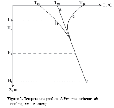
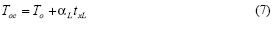
Where T_oa is the mean ground surface temperature at the moment of time t = 0 years; z is the vertical depth and Γ is the geothermal gradient. Is also assumed that the formation is a homogeneous medium with constant thermal properties. Now the current (t = t_x) subsurface temperature is (in case of warming):

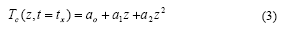
Where a_o, a₁, and a₂ are the coefficients. The temperature-depth values for all wells were taken from the database (Huang and Pollack, 1998; www.geo.lsa.umich.edu/~climate). Four models of changing GST values with time were considered. The corresponding mathematical solutions are presented in the literature (e.g., Carslaw and Jaeger, 1959; Cermak, 1971; Lachenbruch and Marshall, 1986; Lachenbruch et al., 1988; Powell et al., 1988). In the first model (Model C) we assumed that t_xC years ago the GST value suddenly changed from T_o to T_oc. The current temperature anomaly (the reduced temperature) is :

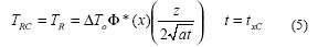
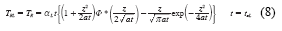
Where a is the thermal diffusivity of formation and Φ*(x) is the complementary error function. In the second model (Model L) we assumed that t_xL years ago the GST value started gradually to change from T_o to T_oc. We assumed that GST is a linear function of time and

Where a_L is some coefficient. The solution is

In the third model (Model S) we also assumed that t_xS years ago the GST value started gradually to change from T_o to T_oc. We assumed that GST is a square root function of time and

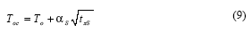
Where a_S is a coefficient. The solution is

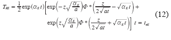
And, finally, in the fourth model (Model E) we assumed that the GST value exponentially increases with time and

Where a_E is a coefficient. The solution is (T_RE=T_R)

Computer programs were used for processing field data and calculating values of t_x, T_oc, T_o, Γ, f(z), a_L, aS, and aE. To demonstrate the calculation technique we present below a field example.

Example of Calculations

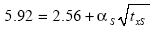
For the interval 49.81-119.58 m of the borehole Ca-9901 (Table 1 and Figure 2) the temperature profile can be approximated by a quadratic equation (standard regression program was applied)

Therefore, the present mean ground surface temperature (GST) is 5.92oC (Figure 1). From the observed T-z data it follows that in the 189.47-596.47 m section of the well; the temperature gradient is practically constant. It was assumed that the temperature gradient in this section did not change. For this interval (here a standard regression program was applied)

Therefore, in the past (t_x years ago) the mean ground surface temperature T_o = 2.56^oC and warming occur.

In our case the observed reduced temperatures (for z < 119.6 m) are:

Where T_obs values are the measured temperatures (Figure 2).

For the calculations below we used the depth z = H1 = 49.81 m, where T_R =1.39 ^oC.

The temperature change (anomaly) of the GST is 5.92^oC – 2.56^oC = 3.36^oC.

A computer program calculates the reduced temperatures versus depth for the four models of change in GST and compares them with the observed anomalies.

For the first model (Model C) the reduced temperature is T_RC (Equation 5). In our case the GST changes from 2.56^oC to 5.92^oC.

In the second model (Model L) the reduced temperature is T_RL (Equation 8) and the ground surface temperature linearly changes from 2.56^oC to 5.92oC, a change that can be modeled using the following equation

In the third model (Model S) the GST is a square root function of time. The reduced temperature is T_RS (Equation 10) and

In the fourth model (Model E) the GST is an exponential function of time. The reduced temperature is T_RE (Equation 12) and

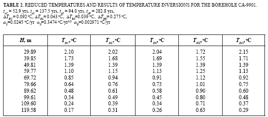
For all models the values of t_x and a were estimated by a computer program. The value of thermal diffusivity a = 0.004 m²/hr was used in the temperature inversions. The results of calculations are presented in Tables 2 and 3, and in Figures 2 and 3.

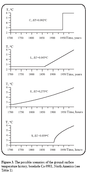
Analyzing the data from Table 2 and Figure 2 we can conclude that the best fit (minimum values of average squared deviations ∆T_RL = 0.043 ^oC and ∆T_RS = 0.039 ^oC) is achieved when the Models L or S are applied.

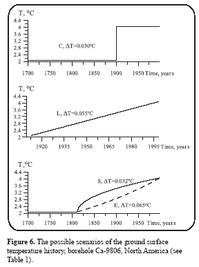
Inversion Results

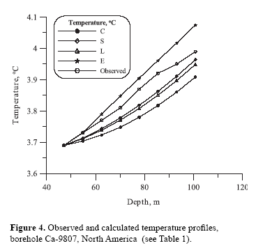
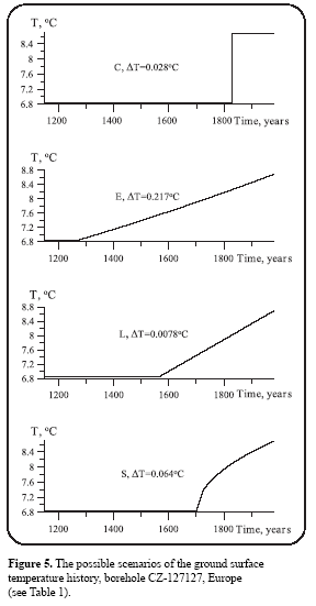
In most cases the Model L (linear increase) and Model S (square root time increase) provide the best fit to the field data (Table 4, Figure 4). In several cases the Model C (sudden change) allows to approximate the measured temperature-depth data with good accuracy (Figures 5 and 6). For boreholes No. 1- 6 (North America, Table 4, Model L) the current warming rates vary in the 0.411- 2.450 K/100a range. The wide range for the warming rate of 0.328-2.482 K/100a was also determined for five boreholes in Europe (Table 4, Model L). Interesting results we obtained for four boreholes in China (Table 4). In this case the warming rate (R_L) varies with relatively narrow limits (1.165- 1.590 K/100a.)

It was found that the duration of warming periods (Table 4, Model L) is: 82-279 years for wells No. 1-6; 99-415 years for wells No. 7-11; and 100-332 years for wells No. 12-15.

Similar results (R_S and t_xS, Table 4) were obtained for the Model S.

DISCUSSION AND CONCLUSIONS

As we mentioned in the Introduction section the main objective of our study is to calculate the warming rates (R) during the 20^th century by the AFR method and to compare with those obtained by the few parameter estimation (FPE) technique (Table 1).

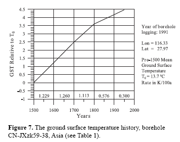
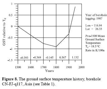
The warming rate estimated by the FPE technique varied in wide ranges: 0.378-2.487 K/100a (North America); 0.212-3.751 K/100a (Europe); and 0.300- 2.532 K/100a (Asia). In our case the FPE method allowed to determine temperature trends (warming or cooling rates) over the past five centuries (Huang et al., 2000). In the inversion we employ a priory null hypothesis for the GSTH that there has been no climate change. From Tables 1 and 4 follows that for the boreholes No. 1-11 (North America and Europe) both approaches (AFR and FPE) provide practically the same ranges of warming rates. For boreholes in Asia (No. 12-15) the AFP technique gives a more consistent (narrow) range of warming rates (1.165- 1.590 K/100a). Let us compare the GSTH of two close spaced boreholes (Figures 7 and 8). Analysis of Figure 7 indicates that the duration of the warming period was five centuries and the warming rate is minimal in the last century. However, it is widely accepted that most of the warming occurs in the last century. At the same time the GSTH reconstructed from borehole No. 12 temperature-depth data (Figure 8) indicates that the cooling period lasted for three centuries and a very high warming rate for the 20th century was calculated by the FPE technique.

The results of temperature inversion by both techniques show that probably some non-climatic effects (well shut-in periods, vertical and horizontal water flows, sedimentation, uplift, erosion, steep topography, lakes, vertical variation in heat flow, lateral thermal conductivity contrasts, thermal conductivity anisotropy, forest fires, farming, etc.) may have perturbed the borehole temperature profiles (e.g., Carslaw and Jaeger, 1959; Lachenbruch, 1965; Kappelmeyer and Haenel, 1974; Powell et al., 1988, Majorowicz and Skinner, 1997; Guillou-Frottier et al., 1998; Kutasov and Eppelbaum, 2003; Gruber et al., 2004; Bodri and Cermak, 2005; Kutasov and Eppelbaum, 2005; Majorowicz and Safanda, 2005; Mottaghy et al., 2005).

This study shows that extreme caution should be used in the selection of temperature-depth profiles for inferring the ground surface temperature histories. A good example in this regard was demonstrated in the study conducted by Guillou-Frottier et al. (1998), where only 10 out of 57 temperature profiles were selected for inversion of the past ground surface temperatures.

We can conclude that only the calculated warming rates for wells in Asia (1.2-1.6 K/100a for Model L or 0.9-1.1 K/100a for Model S, Table 4) can be used for forecasting of short term warming trends.

The authors thank Dr. Raisa Dorofeeva (Institute of the Earth’s Crust, Russian Academy of Sciences (Siberian Branch), and Irkutsk, Russia), Dr. Arkady Pilchin (Universal Geoscience & Environmental Consulting Co., Ontario, Canada) and Dr. John Sánchez, Editorin- Chief of the Earth Sciences Research Journal, for their useful comments and suggestions.

REFERENCES

• Baker, D. G., and D. L. Ruschy (1993). The recent warning in eastern Minnesota shown by ground temperatures, Geophysical Research Letters, 20, 371-374.        [ Links ]

• Beltrami, H., A. M. Jessop, and J.-C. Mareschal (1992). Ground temperature histories in eastern and central Canada from geothermal measurements: Evidence of climate change, Palaeogeography, Paleoclimatology & Palaeoecology (Global Planetary Change Section), 98, 167-183.        [ Links ]

• Bodri, L., and V. Cermak (2005). Borehole temperatures, climate change and the pre-observational surface air temperature mean: Allowance for hydraulic conditions, Global Planetary Change, 45, 265-276.        [ Links ]

• Cermak, V. (1971). Underground temperature and inferred climatic temperature of the past millennium, Palaeogeography, Palaeoclimatology & Palaeoecology, 10, 1-19.        [ Links ]

• Clauser, C., and J. C. Mareschal (1995). Ground Temperature History in Central Europe from Borehole Temperature Data, Geophysical Journal International, 121, 805-817.        [ Links ]

• Gruber, S., L. King, T. Kohl, T. Herz, W. Haeberli, and M. Hoelzle (2004). Interpretation of geothermal profiles perturbed by topography: the Alpine permafrost boreholes at Stockohorn plateau, Switzerland, Permafrost and Periglacial Processes, 15, 349-357.        [ Links ]

• Guillou-Frottier, L., J. C. Mareschal, and J. Musset (1998). Ground surface temperature history in central Canada inferred from 10 selected borehole temperature profiles, Journal of Geophysical Research, 103 (B4), 7385-7397.        [ Links ]

• Harris, R. N., and S. D. Chapman (1995). Climate change on the Colorado Plateau of eastern Utah inferred from borehole temperatures, Journal of Geophysical Research, 100, 6367- 6381.         [ Links ]

• Huang, S., P. Y. Shen, and H. N. Pollack (1996). Deriving century - long trends of surface temperature change from borehole temperatures, Geophysical Research Letters, 23, 257-260.        [ Links ]

• Huang, S., and H. N. Pollack (1998). Global Borehole Temperature Database for Climate Reconstruction, IGBP PAGES/World Data Center-A for Paleoclimatology Data Contribution Series #1998-044, NOAA/NGDC Paleoclimatology Program, Boulder CO, USA, (see also http://www.geo.lsa.umich.edu/~climate, last accessed July 05, 2006.)        [ Links ]

• Huang, S., H. N. Pollack, and P. Y. Shen (2000). Temperature trends over past five centuries reconstructed from borehole temperatures, Nature, 403, 756-758.        [ Links ]

• Jain, S., and R. S. Pulwarty (2006). Environmental and water decision-making in a changing climate, EOS, 87, no. 14, p.139.        [ Links ]

• Kappelmeyer, O., and R. Haenel (1974). Geothermic with Special Reference to Application, Gebruder Borntrager, Berlin.        [ Links ]

• Kutasov, I. M., and L. V. Eppelbaum (2003). Prediction of formation temperatures in permafrost regions from temperature logs in deep wells - field cases, Permafrost and Periglacial Processes, 14, no. 3, 247-258.        [ Links ]

• Kutasov, I. M., and L. V. Eppelbaum (2005). Determination of formation temperature from bottom-hole temperature logs - a generalized Horner method, Journal of Geophysics and Engineering, 2, 90-96.        [ Links ]

• Lachenbruch, A. H., and B. V. Marshall (1986). Changing climate: Geothermal evidence from permafrost in the Alaskan Arctic, Science, 234, 689-696.        [ Links ]

• Lachenbruch, A. H. (1965). Rapid Estimation of the Topographic Disturbance to Superficial Thermal Gradients, Review of Geophysics, 6, 365-400.        [ Links ]

• Lachenbruch, A. H., T. T. Cladouhos, and R. W. Saltus (1988). Permafrost Temperature and the Changing Climate, 5th International Conference on Permafrost, 3, Tapir Publishers, Trondheim, Norway, 9-17.        [ Links ]

• Majorowicz, J. A., and W. P. Skinner (1997). Potential causes of differences between ground and surface air temperature warming across different ecozones in Alberta, Canada, Global Planetary Change, 15, 79-91.        [ Links ]

• Majorowicz, J. A., and J. Safanda (2005). Measured versus simulated transients of temperature logs - a test of borehole climatology, Journal of Geophysics and Engineering, 2, 1-8.        [ Links ]

• Mottaghy, D., R. Schellschmidt, Y. A. Popov, C. Clauser, I. T. Kukkonen, G. Nover, S. Milanovsky, and R. A. Romushkevich (2005). New heat flow data from immediate vicinity of the Kola super-deep borehole: Vertical variation in heat flow confirmed and attributed to advection, Tectonophysics, 401, 119-142.        [ Links ]

• Pollack, H. N., H. Shauopeng, and P.Y. Shen (2000). Climate change record in subsurface temperatures: A global perspective, Science, 282, 279-281.        [ Links ]

• Powell, W. G., D. S. Chapman, N. Balling, and A. E. Beck (1988). Continental Heat-Flow Density, R. Haenel, L. Rybach, and L. Stegena, (Editors.), Handbook of Terrestrial Heat-Flow Density Determination, Kluwer, 167-222.        [ Links ]

• Shen, P. Y., and A. E. Beck (1991). Least squares inversion of borehole temperature measurements in functional space, Journal of Geophysical Research, 96, 19,965-19,979.        [ Links ]

• Shen, P. Y., and A. E. Beck (1992). Paleoclimate change and heat flow density inferred from temperature data in the Superior Province of the Canadian Shield, Palaeogeography, Palaeoclimatology & Palaeoecology (Global Planetary Change Section), 98, 143-165.        [ Links ]

• Shen, P. Y., H. N. Pollack, S. Huang, and K. Wang (1995). Effects of subsurface heterogeneity on the inference of climate change from borehole temperature data: model studies and field examples from Canada, Journal of Geophysical Research, 100, 6383-6396.        [ Links ]