1. Introduction

Energy derived from wind has played a vital role in the history of mankind and is again receiving considerable attention because of its free and non-polluting character. With the development of wind energy technologies and the decrease of wind power production cost, wind power has rapidly developed around the world in recent years (^{Akdag and Guler, 2011}). As a clean energy source wind is considered an alternative to fossil fuels, which actually accelerate global warming. The first scientific research to utilize wind for generating electricity, was initiated by the Danish in the 1960s. The 1973 energetic crisis, forced many governments to realize the value of wind, as a renewable and independent energy source (^{Hanagasioglu, 1999}). Electricity generation using wind energy has been well recognized as environmentally friendly, socially beneficial, and economically competitive for many applications (^{Monfared et al., 2009}). Prediction of wind speed (WS) at the surface or near the surface, is essential in many areas of science and technology, e.g., wind energy generation, aviation, space vehicle launching, weather forecasting, and agro-meteorology (^{Kulkarni et al., 2008}).

Wind field prediction at the level of wind farm, is still a challenging problem. Different methods have been developed (^{Kallos et al., 2007}); and several studies have been performed to estimate the wind potential in different parts of the world (^{Cam and Yildiz, 2006}). There are various strategies for wind speed prediction that can be classified into two categories: (1) statistical methods that can be subdivided into numerical weather prediction (NWP) and persistence and (2) artificial intelligence techniques that have subdivisions such as artificial neural networks (ANN) and fuzzy logic (^{Monfared et al., 2009}).

With the developments made in chaos theory, researchers have looked for the determinism in various seemingly chaotic-looking fluctuations from different disciplines such as physics, chemistry, hydrology, atmospheric sciences, etc (^{Karunasinghe and Liong, 2006}).

The time series prediction is one of the most important aspects in chaos theory. Time series contain much information about dynamic systems (^{Han and Wang, 2009}). These systems are usually modeled by delay-differential equations. Some of them, for example, the ^{Mackey-Glass equation (Mackey and Glass, 1977)}, the ^{Ikeda equation (Ikeda, 1979)}, and equation for an electronic oscillator with delayed feedback (^{Chua et al., 1992}), are standard examples of time-delay systems (^{Bezruchko et al., 2001}).

The main problem of the time series study consist of predicting the next value of a series known up to a specific time, using the known past values of the series. In time series prediction, this is usually first embedded in a state space using delay coordinates:

where x(t) is the value of the time series at time t, t a suitable time-delay and d the order of the embedding. This embedded vector is then used to predict the next value of the series x(t + τ). Therefore, the non-linear dependence of the level of a series on previous data points is of interest, partly because of the possibility of producing a chaotic time series. Note that short-term prediction for chaotic time series have been widely investigated by several techniques (^{Karunasinghe and Liong, 2006}), however, the long-term prediction has not been widely studied in the literature.

In this work, chaotic time series data taken from the Mackey-Glass differential equation were used to develop a neural network. In order to still obtain a more effective correlation and prediction, particle swarm algorithm has been introduced to update the weights of all layers of the network. Next, this hybrid algorithm was used in the long-term prediction of the next 24 and 48 hours of the wind speed time series. To the best of the authors' knowledge, there is no application for the prediction of the wind speed that includes the long-term prediction, such as the one presented here.

2. Computational method

A feed-forward neural network was used to represent non-linear relationships among variables. This ANN was implemented by replacing standard back-propagation algorithm with particle swarm optimization (PSO).

PSO is a population-based optimization tool, where the system is initialized with a population of random particles and the algorithm searches for optima by updating generations (^{Eberhart and Kennedy, 1995}). In each iteration, the velocity of each particle j is calculated according to the following formula (^{Lazzús, 2011}):

where s and v denote a particle position and its corresponding velocity in a search space, respectively. k is the current step number, ω is the inertia weight, ^_c1 and ^_C2 are the acceleration constants, and r₁, ^_r2 are elements from two random sequences in the range (0,1). is the current position of the particle, ; is the best one of the solutions that this particle has reached, and is the best solutions that all the particles have reached. In general, the value of each component in v can be clamped to the range control excessive roaming of particles outside the search space (^{Kennedy et al., 2001}). After calculating the velocity, the new position of each particle is:

The total steps to calculate the output values, using the input values of the network were as follows (^{Lazzus et al., 2014}):

where Xi is the input variables i, and are the smallest and largest value of the data, thus the input data are normalized using this equation. Next, the net inputs (N) are calculated for the hidden neurons coming from the inputs neurons. For a hidden neuron:

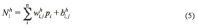
where pi is the vector of the inputs of the training, is the weight of the con n ection among the input neurons with the hidden layer h, and the term corresponds to the bias of the neuron of the hidden layer h, reached in its activation (^{Freeman and Skapura, 1991}). The PSO algorithm is very different from any of the traditional methods of training (^{Lazzus, 2011}). Each neuron contains a position and velocity. The position corresponds to the weiaht of a neuron while the velocity is used to update the weight . Starting from these inputs, the outputs (yi.) of the hidden neurons are calculated, using a transfer function associated with the neurons of this layer (^{Freeman and Skapura, 1991}).

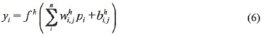
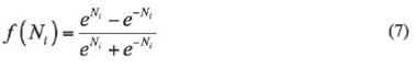
To minimize the error, the transfer function f should be differentiable. In the ANN, the hyperbolic tangent function (tansig) was used as

All the neurons of the ANN have an associated activation value for a given input pattern; the algorithm continues finding the error that is presented for each neuron, except those of the input layer. After finding the output values, the weights of all layers of the network are actualized by PSO, using equations 2 and 3 (^{Lazzús et al, 2014}).

The velocity is used to control how much the position is updated. On each step, PSO compares each weight using the data set. The network with the highest fit ness is considered the global best. The other weights are updated based on the global best network rather than on their personal error or fitness (^{Pérez Ponce et al., 2012}; ^{Lazzús et al., 2014}). In this article, we used the mean square error (MSE) to determine network fitness for the entire training set:

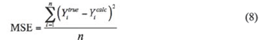
where Yi is the output value obtained from the normalized output (yi) of the network. This process was repeated for the total number of patterns to training. For a successful process the objective of the algorithm is to modernize all the weights by minimizing the total root mean squared error (RMSE):

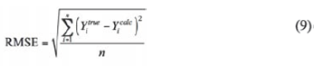
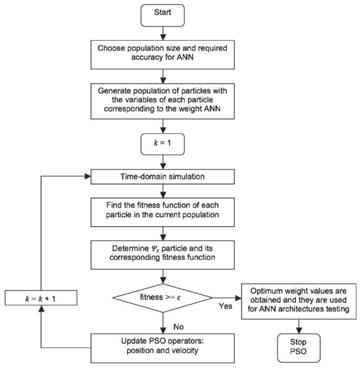
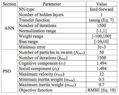
Figure 1 presents a block diagram of the ANN+PSO algorithm developed in this study. In PSO, the inertial weight ω, the constant cl and c2, the number of particles Npart and the maximum speed of particle summarizes the parameters to synchronize for their application in a given problem. An exhaustive trial-and-error procedure was applied for tuning the PSO parameters. Table 1 shows the selected parameters for this hybrid algorithm.

Figure 1 Flow diagram for training of the ANN using PSO algorithm 

Table 1 Parameters used in the hybrid ANN+PSO algorithm. 

3. Simulations

3.1. Mackey-Glass time series

To evaluate the capability of the proposed hybrid algorithm in the long-term prediction, the Mackey-Glass time series was used. Thus, a set of data points were generated from the Mackey-Glass time-delay differential equation (^{Mackey and Glass, 1977}; ^{Farmer, 1982}) which is defined by:

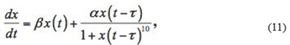
where t is a variable, x is a function of t, and τ is the time delay. The initial values of the time series are α = 0.2, β = 0.1, and x(0)=1.2. If τ ≥ 17, the time series show the chaotic behaviour (^{Farmer, 1982}; ^{Mirzaee, 2009}).

The goal of the task is to use known values of the time series up to the point x=t to predict the value at some point in the future x=t+T. The standard method for this type of prediction is to create a mapping from d points of the time series spaced Δ apart, that is 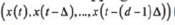to a predicted future value x(t+T).

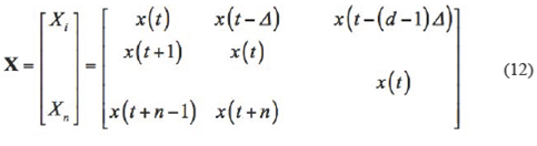
In order to solve the Mackey-Glass equation, the fourth-order Runge-Kutta method was applied to find the numerical solution. The time series was obtained evaluating the solution of eq. (11) at each integer points. Step size of 0.1 was used to generate a time series, and x(t) is thus derived for with in the integration. Four non consecutive points in the time series are given to generate each input vector X. (where i=1, 2, ...,n) of the input matrix X, as:

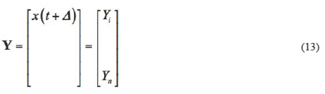
A similar criterion was used to create the output matrix, as:

Then, the ANN+PSO method was used in the long-term prediction. This hybrid algorithm was trained to predict the future value x(t+84) from the current value x(t) and the past values, using the standard form applied in the literature, for d=4 and Δ=T=6 (^{Chng et al., 1996}; ^{Mirzaee, 2009}).

One thousand data points of the above format were collected. The first 500 were used for training while the others were used for testing the ANN+PSO method. Then, the following case was simulated with α = 0.2, β = 0.1, x(0) = 1.2 and τ = 17. From this case, several network architectures were tested.

The most basic architecture normally used for the analysis of chaotic time series involves a neural network consisting of three or four layers (^{Lazzús et al., 2014}). The input layer contains one neuron for each input parameter: x(t), x(t-6), x(t-12), and x(t-16). The output layer has one node generating the scaled estimated value of the chaotic time series x(t+84). The number of hidden neurons needs to be sufficient to ensure that the information contained in the data utilized for training the network is adequately represented (^{Lazzús et al., 2014}). There is no specific approach to determine the number of neurons of the hidden layer, many alternative combinations are possible. The optimum number of neurons was determined by adding neurons in systematic form and evaluating the MSE and RMSE of the sets during the learning process (Pérez Ponce et al., 2012; ^{Lazzús et al., 2014}). For our case the optimum architecture was 4-12-1.

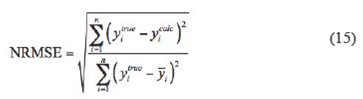
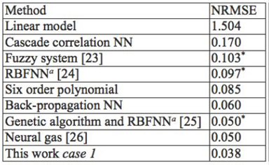
The results obtained with the ANN+PSO method present a MSE=0.000063 and RMSE=0.0079 for training set, and MSE=0.000065 and RMSE=0.0080 for prediction set. These results show that the ANN+PSO model can be accurately trained and that the chosen architectures can predict the long-term x(t+84) with acceptable accuracy. Table 2 shows a comparison between some computational methods found in the literature (^{Martinetz et al., 1993}; ^{Whitehead and Choate, 1996}; ^{Bersini et al., 1997}; ^{Awad et al., 2009}) and the result obtained with the ANN+PSO method. This comparison was made using the normalized root mean squared error (NRMSE), defined as:

Table 2 Comparison between computational methods found in the literature for the long-term prediction. 

*long-term: x (t+85)

^ɑRadial basis function neural network

3.2. Wind speed time series

Once the capability of the hybrid algorithm was proved, it was used to forecast the long-term of wind speed time series.

This study is based in data collected from a meteorological stations located on the semi-arid Norte Chico of Chile (29°54' S; 71°15' W; 10 m), located at south of the hyper-arid Atacama Desert. The region is characterized by complex topography with altitudes varying from sea level until 5000 m at the high Andes Cordillera. The climatic characteristics are influenced by the south-eastern Pacific subtropical anticyclone and the cold Humbolt Current which results in low precipitation rates (^{Kalthoff et al., 2002}). The zone is one of the most sensitive areas in South America (^{Kalthoff et al., 2006}), and recent studies of oceanic and atmospheric variability have confirmed the implications of the dynamics of El Niño-Southern Oscillation (ENSO) cycle on the local climate of this zone (^{Meinen and McPhaden, 2009}).

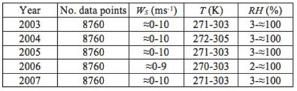
43800 data points (years 2003-2007) were used. The future values of wind speed was predicted using the past values of the time series of wind speed WS(ms^-1), relative humidity RH(%), and air temperature T(K). Figure 2 shows the time series of the selected meteorological data used. The data ranges and the properties of interest are listed in Table 3. As seen in this Table, hourly WS cover wide ranges, going from =0 to 10 (ms^-1). Other wide range for the input parameters are: T from 270 to 305 (K), and RH from 2 to ≈ 100 (%).

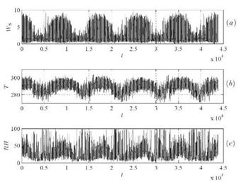
Figure 2 Time series of the meteorological data used in this study. (a) wind speed WS/ms-1, (b) air temperature T/K, and (c) relative humidity RH/%. 

Table 3 Summary of data used in this study. 

The influence of the selected meteorological data in this study (T, RH, and WS) over the climate of the semi-arid zone of the Atacama Desert has been revised and evaluated in other communications (^{Kalthoff et al., 2002}; ^{Kalthoff et al., 2006}). Figure 3 shows WS as a function of the selected meteorological data: T and RH. Fig. 3a shows WS as a function of T with a coefficient of linear correlation (R2) of 0.5979. Fig. 3b shows WS as a function of RH with R2 of 0.2757. Note that the coefficient of linear correlation in this figure shows a non-linear relationship between WS and the input parameters for this climate zone. Then, the relationship between WS and these meteorological data is highly non-linear, and consequently an ANN is the best alternative to model the hourly WS.

Two new cases were studied with this methodology, the long-term prediction of the next 24 hours WS(t+24) and the long-term prediction of the next 48 hour WS(t+48). To select the best input parameters for solving the problem, the hourly data from the current value to 23 past hours (t-23, t-22, t-21,... , t), were considered. Then, the sum of absolute values of weights (SAVW) was used (^{Lazzús, 2013}). Figure 4 shows the input with more contribution for the prediction of future values of Ws This Figure shows the great significance of the past values (t-18), (t-12), (t-6), and the current value (t) on the three meteorological data (W_S T, and RH).

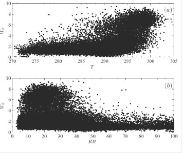
Figure 3 Experimental data of WS from 2003 to 2007 as a function of the selected Meteorological parameters. a) WS vs T → R2=0.5979; (b) WS vs RH → R2=0.2757. 

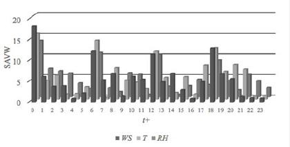
Figure 4 Influence of several points of time series on prediction of future values of wind speed. Bars represent the sumsof absolute values of weights (SAVW) of the ANN+PSO. 

Thus, the optimum input vector was:

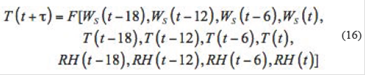
where τ is the future value to predict: 24 and 48 for the long-term prediction.

The leave-20%-out cross-validation method was used to estimate the predictive capabilities of the model. 34996 data points were used in the training set, and 8760 data points (not used in the training step) were used in the prediction set.

4. Results and Discussion

Several network architectures were tested for the long-term wind speed prediction (T(t+24) and T(t+48), separately). The optimum architecture was checked using the objective function (Eq. 10). Figure 5 shows MSE found in correlating the WS as function of the number of neurons in the hidden layer (NN). Fig. 5a shows the best topology found for the prediction of the WS for the next 24 hours T(t+24) with a network architecture 12-28-1. Fig. 5 b shows the prediction of the ^_WS for the next 48 hours 7(/+48) with an optimum network architecture of 12-42-1. Once the best architectures were determined, the optimum weights and biases required to carry out the estimate of future values of ^_WS were obtained.

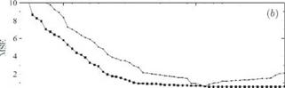
Figure 5 Deviations found in the correlation of wind speed as a function of the number of neurons in the hidden layer for: (a) long-term prediction WS(t+24), and (b) long-term prediction WS(t+48). In both graphics, training step (■) and prediction step (o). 

Figure 6 shows a comparison between real data (black line) and calculated values (points) of long-term prediction of WS(t+24). Fig. 6a shows the forecasting of WS(t+24) with a correlation coefficient (R2) of 0.974 for the training set (years 2003-2006) with a slope of the curve (m) of 0.965 (expected to be 1.0), and with RMSE=0.787 [ms^-1] (MSE=0.620 [m s^-1]² and MSEmax=10.028 [m s^-1]²). Fig. 6b shows the forecasting of WS(t+24) with R2=0.973 during the prediction step (year 2007) with m=0.963 (also expected to be 1.0), and with RMSE=0.807 [ms^-1] (MSE=0.651 [ms^-1]² and MSEmax=7.110 [ms^-1]²).

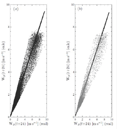
Figure 6 Comparison between real and calculated values of WS(t+24) using the proposed ANN+PSO model. (a) Training set, period 2003-2006; and (b) Prediction set, period 2007. 

Figure 7 shows a comparison between real data (black line) and calculated values (points) of long-term prediction of WS(t+48). Fig. 6a shows the forecasting of WS(t+48) with R2=0.970 for the training set with m=0.963, and with RMSE=0.788 [ms^-1] (MSE=0.622 [ms^-1]² and MSEmax=9.386 [ms^-1]²). Fig. 6b shows the forecasting of WS(t+48) with R2=0.969 for the prediction set with m=0.962, and with RMSE=0.796 (MSE=0.634 [ms^-1]² and MSEmax=8.210 [ms^-1]²).

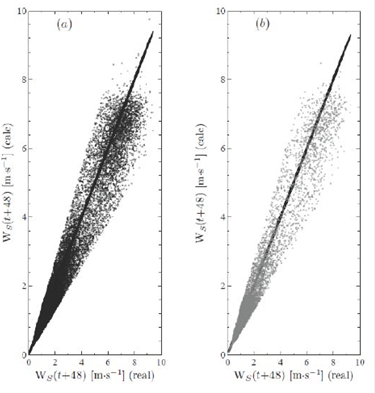
Figure 7 Comparison between real and calculated values of WS(t+48) using the proposed ANN+PSO model. (a) Training set, period 2003-2006; and (b) Prediction set, period 2007. 

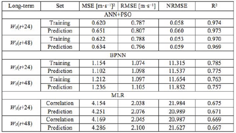
A comparison was made with a neural network with standard back-propagation (BPNN) algorithm (^{Hagan and Menhaj, 1994}), and similar architecture and database. This BPNN show results of MSE higher than 1 [ms^-1]² and R² lower 0.8 for the forecasting of WS(t+24) and WS(t+48). And other comparison was made with a multiple linear regression (MLR) method, and similar database. The MLR method shows MSE higher than 4 [ms^-1]² and R² lower 0.7 for both cases. Note that, the predictions with the proposed ANN+ PSO method shows MSE a little higher than 0.6 [ms-¹]² and R² higher than 0.97. Table 4 summarizes the deviations obtained in the long-term prediction using the proposed method versus BPNN and MLR methods. These results show that the ANN+PSO can be accurately trained and that the chosen topologies can estimate the future values of WS with acceptable accuracy. These results represent a tremendous increase in accuracy for forecasting this important meteorological property and show that not only the optimum architecture obtained was crucial, also the appropriate selection of the independent parameters (T and RH). This is important because air temperature and relative humidity are commonly available parameters. Note that the coefficients of linear correlation of these parameters show a non-linear relationship with the WS for the climate of several geographic zones. Then, the relationship between WS and these meteorological data is highly non-linear, and consequently the ANN+PSO is a good tool for modeling WS for several applications.

Table 4 Summary of the deviations obtained with the ANN+PSO algorithm for the long-term prediction of wind speed. 

The results obtained by other models and other sites can be usefully compared with our results. ^{Zhang et al. (2012)} shows the performance analysis of four modified approaches for wind speed forecasting for four observation sites in Gansu (China), with MSE higher than 2 [ms^-1]². ^{Liu et al. (2013)} shows the forecasting models for wind speed using wavelet, wavelet packet, time series and artificial neural networks with MSE higher than 1 [ms^-1]². For Spain, the wind speed estimation was made using a multilayer perceptron with MSE higher than 1 [ms^-1]² and R² below 0.75 (^{Velo et al., 2014}). Recently, ^{Wang et al. (2014)} shows the mean hourly wind speed prediction in the Hexi Corridor of China based on the seasonal adjustment method (SAM), exponential smoothing method (ESM), and radial basis function neural network (RBFN), with RSME higher than 0.7 [ms^-1]. It must be mentioned that these results were obtained from different sites and based on different weather conditions, and the results cannot be compared directly with one another. However, results from the different methods show that the accuracy of ANN+PSO model employed in this study is good.

5. Conclusions

In this work, a neural network was used for the forecasting of long-term wind speed time series. In order to obtain a more effective correlation and prediction, particle swarm algorithm has been introduced to update the weights of all layers of the network. 43800 data points (years 2003 2007) of wind speed were used. To distinguish between the different values of hourly data considered in this study, so that the network can discriminate and learn in optimum form, the following past values of the time series of meteorological data were used as input parameters: wind speed WS(ms^-1), relative humidity RH(%), and air temperature T(K).

Based on the results and discussion presented in this study, the following main conclusions are obtained: i) The results show that the proposed ANN+PSO can be properly trained for predicting the hourly wind speed, with acceptable accuracy; ii) the meteorological variables used (WS, T, and RH), have influential effects, on the good training and predicting capabilities, of the chosen network; iii) The low deviations found with the proposed ANN+PSO method indicate that it can predict the future values of WS with better accuracy than other methods; and iv) The values obtained with the proposed method are believed to be sufficiently accurate for engineering calculations, among other uses.