


 English (pdf)
 Article in xml format
 Article references
 Send this article by e-mail
 Cited by SciELO
  Cited by Google
  Similars in
SciELO
Similars in
SciELO  Similars in Google
 Permalink
1. Introduction
The introduction of significant amounts of wind energy into power systems makes accurate wind power forecasting as a crucial element of modern electrical grids. Power systems require forecasts with temporal scales of tens of minutes to a few days at wind farm locations. Traditionally these forecasts predict the wind at turbine hub heights, and then they are converted into power output predictions at wind farms. Since the available wind power is proportional to the wind speed cubed, even small wind forecast errors result in significant power prediction errors. Accurate wind forecasts with high temporal scales and spatial resolution at the location of wind farms are significant and essential components in the integration of wind power into power systems.
Numerous efforts have been undertaken to predict the wind at a hub height of large wind farms using numerical weather prediction (NWP) models (Asis et al., 2017; Giebel et al. 2011) or statistical models. NWP models focus on the thermodynamic characteristics of the atmosphere coupling with the complex topography and land cover, which have the temporal scale of a few minutes to a day and horizontal spatial scale of a few kilometers to several hundred kilometers (Lindang, 2017; Pielke, 2002). However, NWP models systematic errors arise from errors in the initial conditions or parameterization. The statistical approach is based on training with measurement data and uses the difference between the predicted and the actual wind speeds in immediate past to tune model parameters, which are more economical regarding computer resources. Usually, statistical methods forecast for lead times shorter than 6 hours and the mathematical relationships should be formulated from the past observation as long as possible. Therefore, NWP model and statistical post-processing models can be combined to accurately forecast the hub-height winds at wind farms in complex terrain (Landberg 2001). The physical models try to use environmental considerations as long as possible to reach the best possible estimate of the local wind speed. Statistical models try to find the relationships between NWP results and observations to reduce the remaining error.
The physical methods (NWP model) differ widely in their model formulations, spatial and temporal resolutions, and parameterizations. Since wind turbines are situated in the planetary boundary layer (PBL), physics options including the PBL scheme and land surface model taking the variation of the wind with height into account are proposed. Wind power statistical models, such as Calman filter algorithm, artificial neural network (ANN, Carolin and Fernandez 2007; Li et al. 2009) and support vector machine (SVM, Yang et al. 2009; Zhang and Zeng 2010) models, have been shown to outperform the conventional statistical models as artificial intelligence methods. The combined statistical models, including 2 or more statistical models, overcomes the limitations of one statistical model and improve the accuracy effectively (Peng et al. 2011). Then, which mesoscale NWP model should be proposed to predict the hub-height winds, how to set up the NWP model, and which post-processing statistical modules could correct the errors, are significant problems and need more study.
This study aims to accurately predict the hub heights (70 m) winds at a wind farm on a plateau located in the Inner Mongolia using a hybrid approach, which combines physical and statistical approach. The Weather Research and Forecasting (WRF) model was used as the mesoscale NWP because WRF is evidenced to have the ability to simulate the near-surface wind even in complex terrain (Lai et al., 2017; Shimada et al. 2011; Deppe et al. 2012). The most widely used planetary boundary layer (PBL) schemes, the Yonsei University scheme (YSU), and the Noah land surface model were combined with the WRF model. The statistical post-processing models were selected to accurate the NWP model output, including persistence (P), back-propagation artificial neural network (BP-ANN) and least square support vector machine (LS-SVM) models. The short-term forecasting (day-ahead), immediate-short-term forecasting (6-h ahead) and nowcasting (1-h ahead) were selected to verify the above dynamical-statistical forecast. This work contributes to a better understanding of the wind conditions and the predictability of the hub-height winds for wind farms.
In section 2, we describe the wind data, the WRF/YSU/Noah, and the statistical models. Section 3 presents the results, which are summarized and discussed in section 4.
2. Data and methodology
2.1. Data
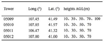
The wind observations are taken from the four meteorological towers (05009, 05010, 05011, 05012; see Table A2) on a wind farm in Inner Mongolia at different height (10 m, 30 m, 50 m, 70 m, and 100 m) with a 10-min time step from 2 January to 31 December in 2010. Based on the homogeneity test, the observations from 2 January to 22 March in 05010 and from 17 March to 22 March in 05011 are removed (Li et al. 2015).
2.2. WRF /YSU /Noah
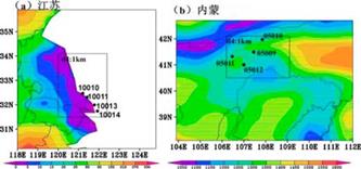
The mesoscale model used in this study is the non-hydrostatic WRF model version 3.3.1 (Skamarock et al. 2008). There are 34 vertical levels with higher resolution in PBL. The top of the model is 50 hPa, and the lowest is 10 m above ground level (AGL). There are 12 levels in the lowest 1 km AGL to improve the vertical resolution in PBL. WRF model is configured with four two-way nested domains with horizontal grid spacing of 27 km (D1), 9 km (D2), 3 km (D3), and 1 km (D4), respectively (Fig. B1). The outermost domain covers the most of China, the South China Sea and some parts of the Pacific Ocean, which provides the background circulation for the inner grid. The private domain covers the research region to simulate the local circulation system (Yu & Rahim, 2017).
Model physics options include the WRF Single-Moment 5-class (WSM5) scheme for microphysical parameterization (Hong et al. 2004), the Kain-Fritsch cumulus scheme (Kain 2004) only for the utmost two domains, the Dudhia (1989) shortwave radiation scheme, and the Rapid Radioactive Transfer Model (RRTM) for radiation (Mlawer et al. 1997). We found PBL schemes and land surface models are important for the reasonable prediction of the near-surface winds. Then the YSU PBL parameterization with the Monin-Obukhow surface layer scheme (Hong et al. 2006) and Noah land surface model (EK et al. 2003) were selected after some examinations (Li et al. 2015).
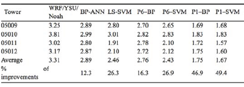
Table 2 Root Mean Square error (RMSE) for different prediction methods and different forecast lengths to 10 day test period from the 20th to 30th of each month in 2010. (Unit: ms-1)
The National Centers for Environmental prediction (NCEP) final operational global analysis (FNL) data on 1.0 x1.0 grids at every six hours are used to initialize the WRF model, which are available on the surface and at 26 pressure levels from 1000 to 10 hPa. The moderate-resolution imaging spectroradiometer (MODIS) land data is adopted which is more close to the actual land surface features. The WRF output is archived at 10-min intervals for analysis. D1, D2, D3, and D4 are activated at 0000 UTC, 1200 UTC, 1800 UTC, and 0000 UTC in the next day, respectively. Then the model integral time of D1, D2, D3, and D4 are 48 h, 36 h, 30 h, and 24 h, respectively. The first 24 h of D1 runs as a spin-up period. The finest domain simulations are used to forecast the turbine hub winds. This forecast experiment covered the time from 2 January to 31 December in 2010.
2.3. Statistical models
(a) Persistence method
Persistence is one of the simplest prediction models and most frequently used in wind energy forecasting. In this model, the forecast for all times ahead is set to the value it has now. The mean relative errors of persistence model for the four sites in 1-hour forecast horizon are shown as Figure B2, which were calculated from the observed 70-m winds during 2 January to 31 December in 2010. The results indicate persistence has a good forecast in a few minutes to several hours ahead. This is because the dominant time scales of large synoptic scale changes in the atmosphere are in several days; then the pressure systems and winds would be changed on the same time scales. Because the relative error of forecast winds is required to be smaller than 20%, the persistence model was used in immediate short-term forecasting and nowcasting.
(b) BP-ANN
The back-propagation algorithm is the most common artificial neural network (ANN), and the learning algorithm is the steepest descent algorithm that minimizes the errors between the produced output and the desired output by adjusting the weights. BP-ANN is based on the error back-propagation learning algorithm, which has the distributed information storage and processing structure, and is suited for short-term forecasting (Carolin and Fernandez 2007; Li et al. 2009). Three-layered BP-ANN can approximate any nonlinear function and shows good performance on handling complex nonlinear problems. Two normalized functions were used in this paper. One is premnmx, which is mainly used to normalize the training set, and another is tramnmx, which is used to normalize the prediction set. The anti-normalized function used in this paper is postmnmx.
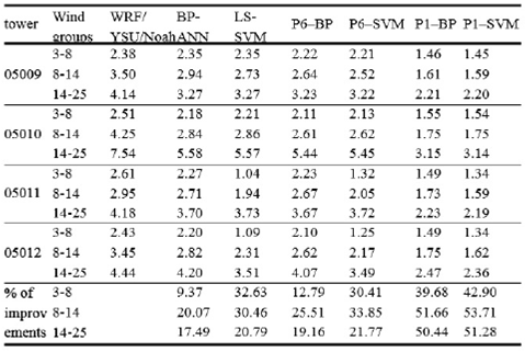
Table 3 RMSE of wind speeds intervals associated with different forecast methods and different forecast lengths to 10 day test period from the 20th to 30th of each month in 2010. (Unit: ms-1).
(c) LS-SVM
Support vector machine (SVM) is a statistical learning theory system based on the Structural Risk Minimization principle and Vapnik-Chervonenkis Dimension theory (Vapnik 1995), which is to map the input data into a higher-dimensional feature space via a kernel function and to construct the optimal hyperplane for classification and regression. LS-SVM works with a sum squared error cost function, uses the equality constraints instead of inequality constraints in conventional SVM and transforms the quadratic programming problem into linear equations, which simplifies and speeds up the calculation and enhances the accuracy of convergence. In this paper, intelligent search of genetic algorithm was employed in the process of choosing parameters of LS-SVM, and to find the optimal model parameters of LS-SVM for different data sets. Compared with the exhaustive search, the performance is improved with less searching times in larger parameter space (Rahim & Usli, 2017).
2.4. hybrid structure
BP-ANN and LS-SVM were used in this paper as statistical correction model for short-term forecasting. Persistence combined with BP-ANN and persistence combined with LS-SVM were used for immediate short-term forecasting (referred to P6-BP and P6-SVM, respectively) and nowcasting (referred to P1-BP and P1-SVM, respectively). To eliminate the seasonal variation of wind speeds, the statistical relationships are trained for each month. Thus the each monthly wind speeds are divided into training (the first 2/3 time series) and validation sets (the last 1/3 time series). The statistical models are trained using the first 2/3 data to learn the relationship between the NWP output wind speeds, and the observations, then use the model parameters to forecast the 70 m winds for the last 10 or 11 days with a time step of 10 min (updates every 10 min). During the training processes, the training vectors are the WRF output wind speeds and the target vectors are the observations, which are both from the 1st to 20th days in each month with a time step of 10 min and the sample number is 2880. During the predicting processes, the testing and target vectors are from the WRF outputs and observations during the 20th to 30th/31th of each month in 1440 sample-numbers, respectively. The combined technique focuses on the variable weight coefficient, which is chosen based on the lowest root mean square error (RMSE) of prediction.
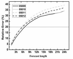
Figure 2 The mean relative error (%) of persistence model for the four meteorological towers, which calculated from the observed 70-m winds during 2 January to 31 December in 2010.
3. Evaluation of 70 m wind forecasts
To test the hybrid approach for 70 m wind forecasts, the WRF/ YSU/Noah wind output, the short-term forecasting (including BP-ANN, LS-SVM), the immediate short-term forecasting (including P6-BP, P6-SVM), as well as the nowcasting (including P1-BP, P1-SVM) were compared using the RMSE as the error measure. Four bias-correction approaches were examined: one based on wind speed only, one using wind speed along with the direction, one based on the diurnal cycle of wind speeds, and the last examine the seasonal variability of wind speeds. The test set using only the validation sets from the 20th to 30th of each month in 2010 was used to determine which bias-correction approach resulted in the lowest RMSE.
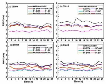
Figure 4 A 24-hour time series of RMSE (unit: ms-1) for wind speed at 70 m AGL associated with different forecast approaches, which calculated from the 20th to 30th of each month in 2010. (a) 05009, (b) 05010, (c) 05011, (d) 05012
3.1. Wind speed evolution
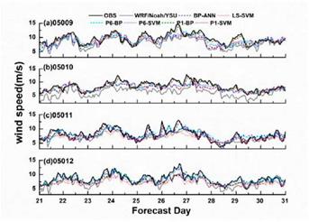
Figure B3 shows the 10 day time series at 1 hour increments of annual average wind speed which were calculated from the 20th to 30th of each month in 2010 based on the WRF/YSU/Noah, BP-ANN, and LS-SVM for short-term forecasting, P6-BP and P6-SVM for immediate short-term forecasting, as well as P1-BP and P1-SVM for nowcasting. The six forecast approaches were found to have under-prediction of the wind speed, and the accuracy of wind speed prediction was decreasing along with prediction time. The WRF/YSU/Noah outputs without any post-processing show the lowest average 70-m wind speeds, which indicates that the NWP model outputs combined with statistical techniques are necessary for wind speed forecast. The six hybrid approaches, BP-ANN, LS-SVM, P6-BP, P6-SVM, P1-BP, and P1-SVM, forecast the 70-m wind speeds in the RMSE of 2.89, 2.46, 2.76, 2.43, 1.75, 1.67, respectively (Table A2). The quality of short-term forecasting, including BP-ANN and LS-SVM, is better than the WRF/YSU/Noah model outputs, which improved the day-ahead forecast in RMSE of 12.3% and 26.3%, respectively. The immediate short-term forecasting shows a 16.3% and 26.9% improvement over NWP output in 70-m wind speed prediction using P6-BP and P6-SVM methods respectively. The nowcasting approaches using P1-BP and P1-SVM exhibits a significant degree of improvement in 70-m wind speed forecasting over the other approaches tested, and the lowest RMSE is 1.75 and 1.67 ms-1 respectively. It is noted that the LS-SVM technique predicts much better than BP-ANN after they were combined with persistence model for the three kinds of 70-m wind forecasting.
The available wind power is proportional to the wind speed cubed, hence the power curve is non-linearity. The available wind speed for a turbine is between the cut-in and rated wind speed (3-25 ms-1). When the wind speed is in the range of 3-8 ms-1 the wind turbine is gradually running, and the production power rises slowly; when it reaches 8-14 ms-1, the production power increases rapidly; and if it reaches 14-25 ms-1, the wind energy is stable. Therefore, to understand the different issues involved in 70-m wind forecasting it is useful to divide the wind speed into three distinct groups: (1) 3-8 ms-1; (2) 8-14 ms-1; (3) 14-25 ms-1. Table A3 shows the RMSE of wind speed groups associated with different forecast methods and different forecast lengths, which indicates the RMSE of wind speed prediction is increasing along with stronger wind speed. The improvement in RMSE of the 70-m wind speed forecast is in the range of 9.4% to 32.6% in short-term forecasting, 12.8% to 33.9% in wind speed forecast in the range of 8-14 ms"1, which is just associated immediate short-term forecasting, and 39.7% to 53.7% in nowcasting. It with the fastest growth of turbine output along with the wind speed. should be noted that such forecast technique significantly improves the wind speed forecast in the range of 8-14 m·s-1, which is just associated with the fastest growth of turbine output along with the wind speed.
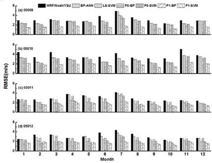
Figure 5 The monthly RMSE (unit: ms-1) for wind speeds at 70 m AGL associated with different forecast approaches, which calculated from the 20th to 30th
3.2. Diurnal cycle of wind speeds
Figure B4 shows a 24-hour time series of RMS for wind speed at 70 m AGL associated with different forecast approaches in the training sets. The mountainous terrain of the Inner Mongolia Plateau is complex with a strong turbulence, then the daily variation of the wind speed is different for different sites. But even that, all physical-statistical approaches exhibit a significant improvement in wind forecast and present the similar error in the diurnal cycle. The WRF/YSU/Noah outputs have the largest error in RMSE, and the nowcasting have the lowest. For the short-term forecasting, WRF/YSU/ Noah coupling BP-ANN and LS-SVM has the similar bias-correction on the station 05009, and 05010, whose error curve in RMSE is consistent with the cure of WRF/YSU/Noah output. But for the station 05011 and 05012, the forecast ability of WRF/YSU/Noah coupling LS-SVM is better than coupling BP-ANN obviously. The immediate short-term wind speed forecastings also develop the forecast error compared to the short-term forecasting, and the two error cures (P6-BP, P6-SVM) are almost the same.
3.3. Seasonal variability of wind speeds
To test the forecast skill on seasonal variability, the monthly RMSE for 70-m wind speeds of different forecast approaches is shown in Figure B5. What the results also agree with the conclusion that the accuracy of wind speed prediction is decreasing along with prediction time and the now casting is better than other time-scale forecasts (Shuib, et al., 2017). The three time-scale wind speed prediction in RMSE is between 1.2 to 4.9 ms-1. Also, the accuracy of wind speed prediction is smaller in autumn and larger in spring and summer. The relative largest RMSE is in July and the smallest in October. Furthermore, for the same time-scale forecasts, the method using LS-SVM forecast wind speed is better than that using BP-ANN.
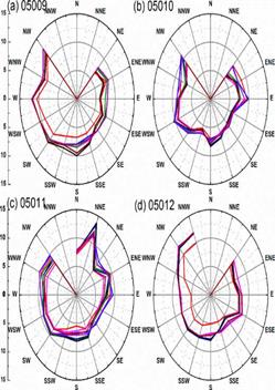
3.4. Wind speed rose diagram
The wind direction is an important factor to be considered in wind power generation. The observation and forecast wind data were averaged over the 15-day test period to generate the wind speed rose, plotted at a 22.5-degree angular resolution and in 5 ms-1 intervals in wind speed, illustrated in Figure B6. The value represents the average wind speed in the 16 different wind directions. As can be seen that all the wind speed roses illustrate a valley in the about northerly direction. The WRF/YSU/Noah outputs exhibit the lower 70-m wind speed at the four sites than other forecasts (Roslee, et al., 2017; Ridzuan et al., 2017). The three time-scale forecasting successfully forecast the westerly (from SSW to NNW) speed at 05012, and the nowcasting shows a significant degree of improvement in wind speed forecasting at all four sites. The error of immediate short-term forecasting is between nowcasting and short-term forecasting. Although the different approaches have different improvement on the different stations, the hybrid forecasting with physical forecasting and statistical postprocessing could predict the wind much better.
4. Summary
The wind energy forecasting problem is closely linked to the problem of forecasting the variation of winds over very short time intervals because the wind is variable and intermittent over various time-scales. To understand the different issues involved in 70-m wind forecasting, the four wind towers in the Inner Mongolia were used to represent the complex plateau terrain, and it was useful to divide the problem into three difference time scales: short-term, immediate-short-term, and nowcasting. The mesoscale WRF/Noah/YSU as the NWP model performed 24-h wind forecast with 1-km horizontal resolution and 10-min time resolution. BP-ANN and LS-SVM were used to short-term forecasting. Persistence method was combined with BP-ANN and LS-SVM to forecast the immediate short-term forecasting and nowcasting, respectively. The results indicate that the current forecasting techniques exhibit considerable skill in short-term, immediate-short-term, and nowcasting forecasting. Short-term forecasts typically outperform an NWP forecast by 12% to 26%; nowcasting forecasts usually outperform NWP forecasts by 47% to 50%.
This paper also demonstrates that the approaches using LS-SVM model is more accurate than the approaches using BP-ANN model over the different time-scales tested. The possible reasons are as follows: 1, SVM is proposed for problems with limited samples to obtain the global optimum solution. 2, SVM algorithm can transform the problem into a quadratic programming problem to obtain the global optimum solution which BP-ANN cannot achieve. 3, SVM uses the nonlinear transformation to map the original variables to the higher dimensional feature space to construct the linear classification function, thus ensuring the good generalization ability of the model, and then avoids the Curse of Dimensionality.

