


 English (pdf)
 Article in xml format
 Article references
 Send this article by e-mail
 Cited by SciELO
  Cited by Google
  Similars in
SciELO
Similars in
SciELO  Similars in Google
 Permalink
1. Introduction
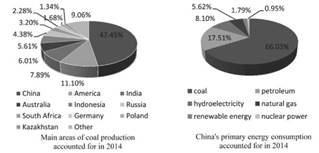
China is the largest producer of coal in the world because coal plays an essential role in the economic development of China (Figure 1). Coal mining accidents have become a frequent occurrence in recent years (Zhang et al., 2014; Wang et al., 2016). Although the death rate resulting from these accidents in China has declined, it is still 70 times higher than that in the United States and 17 times higher than that in South Africa. Against this backdrop, it is urgent to study how to find effective ways to detect water quantity in the aquifer and reduce coal mining accidents (Zhang et al., 2015). Among some geophysical methods currently available, TEM technology is one that has received much attention and has been widely used to reduce coal mining accidents.
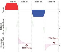
In a TEM application, an ungrounded loop-line first transmits downward a pulse-type primary field, which induces an eddy current. The spatial and temporal distribution of a secondary field caused by the eddy current can then be observed through the coil (Yu, 2007; Wang et al., 2011; Tanaka and Kunisada 2011). By measuring the variation rule of the secondary magnetic field over time during the time-off period, the geoelectricity features at different depths can be obtained (Guillemoteau et al., 2011; Tuncer et al., 2014). From Figure 2 it can be seen that TEM receives induced signals during the time-off period, which will be attenuated over time.
By using the TEM method, we can solve some geological problems (Cheng et al., 2013; Hu et al., 2013). Due to its features such as light equipment, little lateral influence, and high resolution, TEM can be widely applied in water disaster prevention and control (Zhang et al., 2010; Mollidor et al., 2013; Xue et al., 2013; Tao et al., 2013). However, because of the focus on theory development and processing method restraints, past analyses have usually been qualitative, which cannot meet the standard of quantification, and, to certain extent, hinders the application of TEM on a wider basis(Xu et al., 2012; Wang et al., 2014). Hence, in this study, we will develop a theory and propose a method to calculate TEM responses. To do so, we will use equivalent substitution, interpret the diffusion law of TEM field from the perspective of physics, calculate physical parameters, and conduct 3D apparent resistivity imaging and quantitative analyses of detection results.
2. TEM Data Processing
2.1. Apparent Resistivity Calculation
The transmitting loop center induction electromotive force  of horizontal round loop in uniformity whole space medium is:
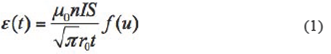
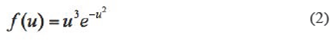
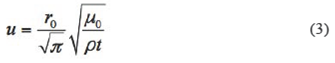
Where µ0 is the vacuum permeability, n is the turn number of transmitting loop, I is the respective emission current, S is the receiving loop similar area, r 0 is the transmitting loop radius, / is the observation time and ρ is the true resistivity of the medium.
From Equation (3), we can obtain an equation as below:
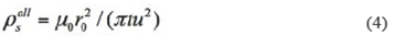
If the loop forms a square about
b
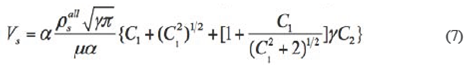
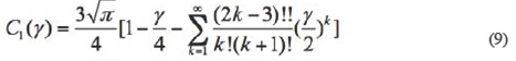
meters on a side, and  , then, with Equations (1) ~ (4), the all-time apparent resistivity
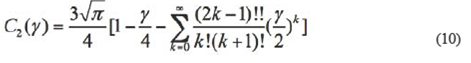
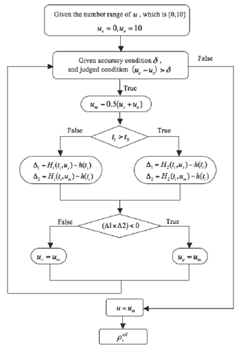
  can be calculated with the binary search algorithm. The calculation process is illustrated in Figure 3.
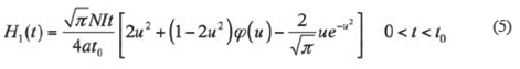
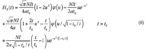
For any observation window t, u is set as [0,10], and the searching region of u can be seen as an absolute value, and among them, us is the initial value of the searching region, ue is final value, ue is a median value which is u value. u is calculated by a binary search algorithm. is actual measured magnetic value, and H(ti) is:
2.2. Depth Conversion
The detection depth D of the TEM method is related to transmitting magnetic torque, all-time apparent resistivity, and the minimum resolutive voltage. The time-depth conversion equation for mine-oriented TEM method is:

where α is the conversion coefficient, which is about the heterogeneous conductor in the vicinity of the roadway and usually values between 0.6 and 1.8; β is the factor of proportionality and  . where
ρi
is the corresponding resistivity value of moment
ti
.
. where
ρi
is the corresponding resistivity value of moment
ti
.
2.3. Interpolation Operation
Due to the unstable workload, the measured and computational data of experiment and field are always not accurate enough, so interpolation is introduced as a supplement.
K(xk
,
yt
,
zt
) is an arbitrary point in the three-dimensional space. There is given pointy 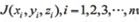 , which is the vicinity of K. The inverse distance weighting method can be used to attribute the value
XK with the equation:
Where di is the distance between the interpolating point and the given point in the vicinity. Yk and Zk can be calculated in the same way as Xk.
2.3. 3D Slice Extraction
3D visualization is a technique to reveal and describe spatial data, receive the subsurface geological structure and features, which provides information for accurate description of the 3D geological structure, and facilitate the exploration and development of coal mine.
According to the data received from different detection directions, it can be seen that 3D visualization can clearly display the spatial distribution of anomalies with different resistivity values that correspond to different threshold values, the scattered points, and the range of apparent resistivity. However, a cross-section map can be clearer in showing the anomaly areas at a particular depth on a profile. Cross-sections can be extracted from different depths of Plane XY, YZ, and ZX. Apparent resistivity data can be extracted from any depth or vertical profile.
2.4. Aquifer Water Quantity Estimation
Through the cross-section map, the aquifer water volume can be calculated with the followino formula:
In this equation, Q is the aquifer water quantity, K is the water containing coefficient, M is the aquifer thickness, and S is the water-rich area in the aquifer.
3. Field Application
3.1. Geological Setting
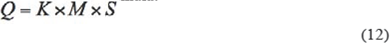
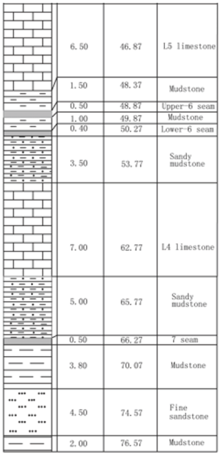
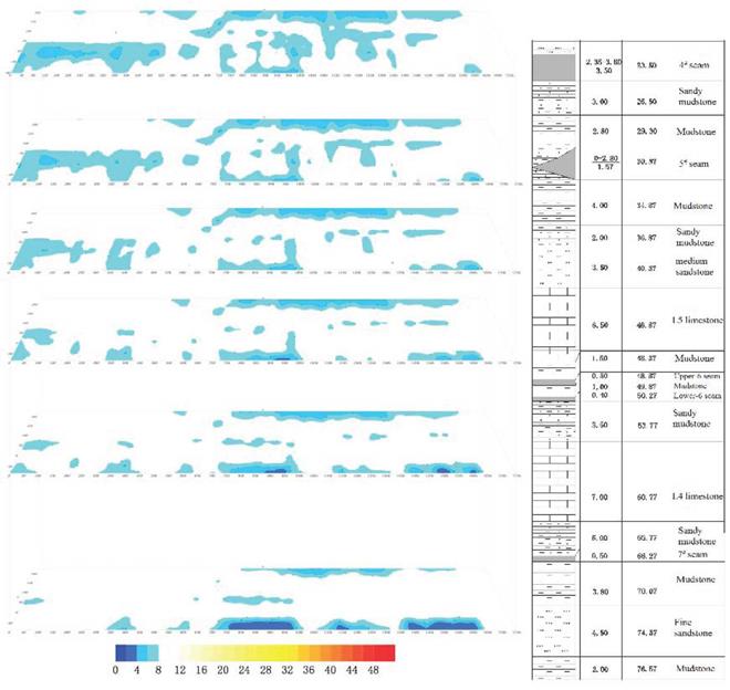
The No.80101 Workface of Jude Mine in Shanxi Province is under L1 limestone in the middle and lower part of Taiyuan formation, 60.6m beneath the 4# seam. The seam occurrence is stable with a thickness range of 1.8 to 3.2m, and a 2.8m thickness on average. Part of the area contains a 0.05 to 0.1m dirt band of mudstone or carbonolite (carbonaceous mudstone). At the bottom of the seam is a pyrite seam in forms of lamella and nodule. The lithological column is shown in Figure 4.
3.2. Field Detection
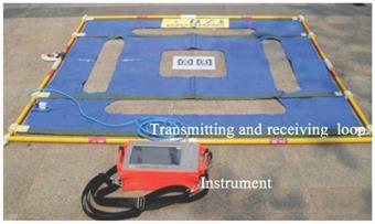
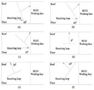
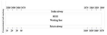
To detect the spatial distribution of the goaf and estimate the water quantity, MTEM was adopted with the YCS360 Electromagnetic System (as shown in Figure 5). The detection of the No.80101 workface starts at the intersection of the return airway and the concentrated rail roadway, then goes on from the return airway to the openoff cut, and ends at the intersection of intake airway and concentrated rail roadway. The total detection workload is 3470 m, including 1660 m along the return airway, 150 m in the openoff cut, and 1660 m along the intake airway. Monitoring points are set every 10 meters, and the detection is conducted in 6 directions, including 60°, 45°, and 30° to the external wall roof, standard to the ceiling, and 30° and 45° to the interior wall roof. The TEM detection direction diagram is shown in Figure 6, and the arrangement diagram of MTEM is shown in Figure 7.
3.3. Data Interpretation and Result Analysis
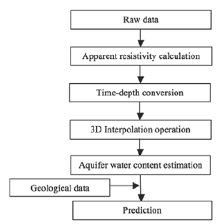
The data is processed based on the standard flow chart (Figure 8), and data interpretation is carried out from the perspective of geophysical characteristics. The features are shown in 3D images. Water quantity is higher in areas where the fractures are concentrated, indicated by higher electrical conductivity and lower resistivity (i.e., high potentiallow resistivity) anomalies. This characteristic identifies aquifer areas as those where roof resistivity is less than 3Ω.m.
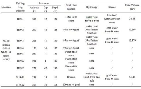
Figure 9 is a 3D spatial distribution graph of anomalies at different depths above the No.80101 workface. 40 meters above the roof is a water-rich stratum, and key preventions should be focused on Region YC1, YC7, and YC10. Anomaly area YC7 is located between 1085m and 1850 m along the return airway (between monitoring point KF13 to KF15), 0-120m along the inclination slope (120m within return airway and workface), and 40m to 60m above the roof (more details in Fig 9), with an anomaly-impacted area of 22,383 m2. The goaf water-filling coefficient is 0.25 to 0.35, and the detection result of the actual ratio is 0.3. It is indicated by the effect sketch that M is 5m, based on the equation Q=KMS. Thus we can deduce that Q=33,574m3. The verification of the calculated values based on field measurements is shown in Table 1. H19-2, H19-3 and H19-S1 boreholes have been constructed for the later next and drainage project, which results in a total water quantity of 33,089m3, and the error percentage of the predicted water volume is less than 1.5%.
4. Conclusions
TEM resistivity imaging boasts rapid imaging, high quantification level, and high resolution, especially when it comes to detecting low resistivity body with a high-resistivity overlayer. With the projection area S of low-resistivity anomaly zone, the water containing coefficient K and the aquifer thickness M, the aquifer water quantity can be estimated with an error percentage of the predicted water quantity below 2%. The TEM 3D presentation and analysis has offered a new method to determine the water amount in an aquifer.

