English (pdf)
 Article in xml format
 Article references
 Send this article by e-mail
 Cited by SciELO
  Cited by Google
  Similars in
SciELO
Similars in
SciELO  Similars in Google
 Permalink
Introduction
Positional information about natural and man-made features is shown on maps as coordinates. Hence, coordinates has become an indispensable representative means for accurately mapping out natural resources. For example, the geologist needs coordinate to carry out geological mapping, while the drilling engineer require the position to be drilled as well as the azimuth the drilling should be done. In view of the foregoing discussion, it is clear that accurate positional information should be provided for proper planning, management and decision making.
In view of the above, Global Navigation Satellite Systems (GNSS), particularly, Global Positioning System (GPS) have been widely adopted in geospatial sciences and its related Earth Science disciplines for geodetic purposes. Since its arrival, GPS has become an essential technology that has revolutionized data collection and surveying practices at large. However, for the GPS data to be used locally so that compatibility could be created between maps and other geospatial data produced in the national datum, there is a need to perform coordinate transformation (Featherstone, 1996; Yang, 2009). In doing this, Earth Scientist can comfortably apply the GPS measurement locally with minimal degree of errors that are usually created due to different datum size, shape and origin between the national data (non-geocentric) of countries and the global datum (geocentric) of the GPS.
As a means to accomplish such task, empirical based coordinate transformation equations have widely been used. Notable among them is the three-dimension (3D) conformal transformation models like Bursa-Wolf (Bursa, 1962; Wolf, 1963), Molodensky-Badekas (Molodensky et al., 1962; Badekas, 1969), Abridged Molodensky (Molodensky et al., 1962) and Veis (Veis, 1960). Conversely, in recent times, artificial neural network (ANN) techniques have also been applied for coordinate transformation (Gullu, 2010; Gullu et al., 2011; Lin and Wang, 2006; Mihalache, 2012; Tierra et al., 2008, 2009; Tierra and Romero, 2014; Turgut, 2010; Yilmaz and Gullu, 2012; Zaletnyik, 2004; Konakoglu and Gökalp, 2016; Konakoglu et al., 2016; ElSayed and Ali, 2016; Ziggah et al., 2016; Ziggah et al., 2017a). It was, however, evident in literature that, the statistical test called the hold-out cross-validation has been the most commonly used technique to evaluate coordinate transformation models performance. In this hold-out cross-validation method, it was noticed that, most authors are primarily concerned with randomly partitioning the available data into two disjunct samples: a training set and a testing set. Here, the training set is used to determine transformation parameters in the case of the empirical models and for ANN model construction. The testing data, on the other hand, is used to measure the predictive accuracy and stability of the chosen trained ANN model, and the empirical model developed with respect to the transformation parameters computed.
However, many studies have reported some significant limitations for using the hold-out cross-validation procedure. One of the main issues is related to how appropriate the available data set is divided (Reitermanová, 2010). It has been indicated that partitioning the data into training and testing sets reduces the number of samples for calibrating the model, and the results produced is based on the unsystematic chosen split (train, test) sets. Moreover, improper data separation could lead to an unreasonably high inconsistency of the model performance. By virtue of this, any bias resulting from the improper split of the data set could have an adverse effect on the model performance (Kohavi, 1995).
Besides, the hold-out cross-validation method heavily depends on having large datasets making it unsuitable to be applied in data-insufficient situations (sparse dataset). The reason being that in sparse dataset, a single train-and-test experiment performed could yield unstable estimates that do not provide enough convincing evidence of the models generalization ability. This could be attributed to: (i) the inadequate amount of observational data available; (ii) unsuitable train-test split selected; and (ii) high variance of the model performance (Bengio and Grandvalet, 2004). In continuance of this, there is often not enough data for holding some of it for testing purposes in sparse data situation.
To combat these defects, the use of K-fold cross-validation (KCV) technique has been recommended (Burman, 1989; Reitermanová, 2010; Kohavi, 1995). It is for these reasons that this study applied for the first time, the KCV technique to evaluate the coordinate transformation performance of the widely used ANN (radial basis function neural network) as well as the similarity model (Bursa-Wolf).
The present authors were also motivated to apply the KCV approach on Ghana geodetic reference network data for several reasons. First, the ANN approach has only been tested for transforming coordinates between two local geodetic data, namely Accra and Leigon data in Ghana. This can be found in Ziggah et al. (2016). In their study, only 27 local common points were available. Although the data is quite small, the hold-out cross-validation procedure was implemented where 20 co-located points were used to form the model and 7 evenly distributed points were used to test the model. In addition, Ziggah et al. (2017a) developed an error compensation model based on ANN capable of improving the performance of the geocentric translation model. Here, 19 co-located points were divided into 11 training points and 8 testing points, respectively. Due to data limitation, it is suggested by the present authors that the KCV technique may have been more appropriate to represent the true reflection of the ANN performance. It is important to note that no such kind of study has also been carried out in Ghana using the ANN approach to directly transform coordinates between the global datum and Ghana's local geodetic datum.
In continuance of that, the widely adopted GNSS for geodetic purposes has necessitated the transformation of its data to the local datum to make it applicable. In line with that, the present study applied the ANN approach which usage in Ghana for global to local datum transformation has been hampered due to limited data availability. In addition, the similarity, affine and projective transformation models (Ayer, 2008; Ayer and Fosu, 2008; Dzidefo, 2011; Ziggah et al., 2013a, b; Kumi-Boateng and Ziggah, 2016; Anann et al., 2016; Laari et al., 2016; Ziggah et al., 2017b) which have been utilised in Ghana's geodetic reference network could be compared with the ANN via KCV approach. The study will further serve as the foundation for exploiting KCV as an alternate way of assessing transformation models performance in Ghana geodetic reference network.
Study Area and Data
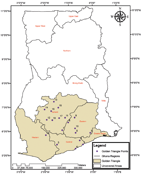
This study was carried out in Ghana, located in the Western part of Africa (Fig. 1). It lies between latitudes 4°30' N and 11o N, and between longitudes 3o W and 10 E. It has a land area of 238, 540 km2 (Fosu et al., 2006) with the highest elevation range not exceeding 880 m above mean sea level located at mountain Afadjato in the Volta Region (Berry, 1995). The land has general characteristics of low grassland and savanna with a divided plateau at the South-Central part of the country (Baabereyir, 2009). Ghana shares border with Ivory Coast to the West, Togo to the East, Burkina Faso to the North and Gulf of Guinea to the South.
The local ellipsoid used in Ghana for its mapping and surveying undertakings is the War Office 1926 suggested by the British War Office. The War Office 1926 ellipsoid has a semi-major axis a = 6378299.99899832 m, semi-minor axis b = 6356751.68824042 m, and flattening f = 1/296 (Ayer, 2008; Poku-Gyamfi, 2009; Mugnier, 2000). The Ghana coordinate system is a projected grid coordinates based on the Transverse Mercator. The origin of the Transverse Mercator is longitude 01o 00' W (central meridian) and latitude 04o 40' N with 274319.736 m as the false Easting added to all Y coordinates to avoid negative coordinates and the false Northing set to zero. A scale factor of 0.99975 is used at the central meridian so that the scale distortion exceeds the projection values only at the extreme ends of the country (Mugnier, 2000). Therefore, positions of features of all survey maps in Ghana are the projected grid coordinates of Easting and Northing derived from the Transverse Mercator 10 NW.
For Ghana to capitalise on the potential of GNSS technology, the Ghana Survey and Mapping Division of Lands Commission with funding from the World Bank and other stakeholders embarked on the Land Administrative Project (LAP). One of the major aims of the LAP is to establish a nationwide GNSS reference network for Ghana. The LAP has been divided into three phases namely the Golden Triangle, Northern triangle and the Kintampo link, and the nationwide coverage (Poku-Gyamfi, 2009). Currently, it is only the Golden Triangle phase covering five out of the ten administrative regions in Ghana that has been completed (Fig. 1). The Golden Triangle (Fig. 1) was strategically established in these five regions due to their massive contributions to the country's economic growth. This is because almost all the natural resources like gold, oil, timber, cocoa, diamond, manganese, bauxite, limestone to mention but a few are located in these regions (Poku-Gyamfi, 2009). The Golden Triangle comprises of three permanent reference stations fixed at the apex of the three largest cities situated at the Western, Ashanti and Greater Accra regions. The reference stations form a triangle of sides 200 km and radii coverage of 100 km with area coverage of 79857 km2 representing 33.5 % of the total land area (238,540 km2) for Ghana (Fosu et al., 2006).
In the establishment of the GNSS reference network, a continuous twelve-hour observation was made on 19 historical triangulation stations located in the Golden Triangle by dual frequency GPS receivers. The coordinates provided by the GPS receivers were then differentially processed with the International GNSS permanent stations to obtain the respective common points on the WGS84 ellipsoid. These 19 satellite coordinates are defined in the International Terrestrial Reference Frame 2005 specified at epoch 2007.39 (Kotzev, 2013).
Data used for the study is from the LAP comprising of 19 Golden Triangle common points on the War Office 1926 (φ,λ, h) WAR and WGS84 (φ,λ,h) WGS84 reference frames. Here, φ is the geodetic latitude, λ is the geodetic longitude and h is the ellipsoid height. It is imperative to note that the local geodetic network of Ghana involves data in geodetic latitude, geodetic longitude and orthometric height (H) without the existence of ellipsoidal height. This, however, impedes the direct conversion of geodetic coordinates to cartesian coordinates. In view of this, the Abridged Molodensky transformation model (Molodensky et al., 1962) was applied in the LAP to get the War Office ellipsoid heights. This was done by applying the Abridged Molodensky model to estimate the ellipsoid correction factor (∆h) between the WGS84 and War Office 1926. The War Office 1926 ellipsoid height (h WAR ) was then calculated using the relation h WAR h= WSG84 −∆h
Methods
Conversion of Geodetic Coordinate to Cartesian Coordinate
The common points geodetic coordinates, (φ,λ,h) wgs84 and (φ,λ,h) war on WGS84 and War Office 1926 was converted to cartesian coordinates (X, Y, Z) using the standard forward equations from Heiskanen and Moritz (1967). The rectangular coordinates derived from the conversion is designated in this study as (X, Y, Z)WGS84 and (X, Y, Z)WAR respectively.
Similarity Transformation Model
This study applied the 3D similarity model of Bursa-Wolf (Bursa, 1962; Wolf, 1963) to transform coordinates from WGS84 to War Office 1926. The Bursa-Wolf model considers the misalignment of the X, Y, Z axes between two reference systems. The Bursa-Wolf model is made up of three rotations, three translations and a scale factor which in totality form a seven parameter transformation approach. One important characteristic feature of this model is that the shape of the geodetic network containing the coordinates to be transformed is preserved, hence angles are not altered after transformation, but the distance between the transformed coordinates and their original positions could be changed (Constantin-Octavian, 2006; Ghilani, 2010).
Mathematically, the Bursa-Wolf model integrates two sets of three-dimensional (3D) rectangular coordinates defined in two different coordinate systems using Equation 1.
where (X, Y, Z)WGS84 and (X, Y, Z)WAR are the respective rectangular coordinates for WGS84 and War Office 1926 ellipsoid. The (TX, TY TZ) are the translations along X, Y, Z-axes of the two reference systems, η is the scale factor and R is the total rotation matrix, respectively. Expansion and simplification of Eq. (1) into least squares form can be found in (Deakin, 2006).
In this study, the total least squares (TLS) approach was used to determine the unknown transformation parameters. The solution of the TLS was done using singular value decomposition (SVD) method. Here, the SVD was first applied on the augmented matrix [A:F]. Here, A is the design matrix and F is the observation matrix. The SVD on augmented matrix [A:F] could be defined by Equation 2 (Golub and Reinsch, 1970; Van Huffel and Vandewalle, 1991; Markovsky and Van Huffel, 2007) as
Where

The σ are the singular values of A and [A:F], and the vectors u
i
and v
i
are the ith left and right singular vector of A and [A:F], respectively. A TLS solution exists if and only if V22 is non-singular and the solution is unique if and only if σ
n
≠ σ
n+1. The TLS(
 ls
) solution for the unknown parameters was determined using Equation 3.
ls
) solution for the unknown parameters was determined using Equation 3.

The corresponding TLS correction matrix (∆C tls ) is given by Equation 4 as

Radial Basis Function Neural Network
The basic radial basis function neural network (RBFNN) structure consist of highly interconnected neurons arranged into three layers: input, hidden and output layer respectively, as shown in Figure 2 where (X1 X2, ..., Xi) is the input layer data and (Y1 ... ,YK) is the output layer target. The input layer accepts the input variables of the problem to be solved and deliver straightforwardly to the hidden layer without weighting.
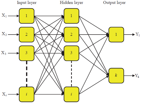
The obtained input data in the hidden layer are then transformed by weight multiplication and the results moved into a nonlinear system by means of a radial basis function (RBF). The most generic RBF widely used in RBFNN known as the Gaussian function was applied in this study. This type of RBF is highly characterized by a centre position and a width parameter which regulates the amount of decrease of the function during training.
The Gaussian function (Jain et al., 2011) is defined in Equation 5 as
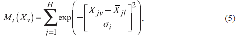
where M¡ (X
v
) denote the hidden layer output value of the ith unit, H is the number of RBF units, X
jv
is the jth variable of the input data v,
 j¡
is the centric position of rth RBF unit for input variable j and σ
i
is the spread parameter of th RBF unit. It should be noted that, in the course of RBFNN training, the RBF parameters (Eq. (5)) are optimized and determined in a three-step procedure. First, the Euclidean based clustering technique is applied to determine the RBFs centres. The spread parameters are then calculated by the nearest neighbour method. To this end, the weights (w) linking the hidden layer neurons (RBF units) and the output layer are estimated using a linear regressor. The estimated output layer results for the RBFNN could be given by Equation 6 as
j¡
is the centric position of rth RBF unit for input variable j and σ
i
is the spread parameter of th RBF unit. It should be noted that, in the course of RBFNN training, the RBF parameters (Eq. (5)) are optimized and determined in a three-step procedure. First, the Euclidean based clustering technique is applied to determine the RBFs centres. The spread parameters are then calculated by the nearest neighbour method. To this end, the weights (w) linking the hidden layer neurons (RBF units) and the output layer are estimated using a linear regressor. The estimated output layer results for the RBFNN could be given by Equation 6 as

where H is the number of radial basis function, w i is the output weight that matches to the association between a hidden node and an output node, while w o is the bias. M ¡ (X v ) is defined in Equation 5.
The mean squared error (MSE) for the vth data is then estimated using Equation 7.
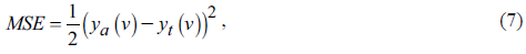
where y α (v) and y t (v) are the actual output and target for the vth data, respectively. Repeat the training process until the RBFNN reach the desired error value. The error function Equation 8.
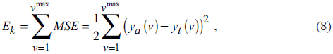
where vmax represents the total number of training data. The optimum trained RBFNN model was then tested using a test data (untrained).
It important to note that, in order for us to carry out the RBFNN training described, both the input and output data were first scaled into the interval [-1, 1] using Equation 9 (Mueller and Hemond, 2013). Scaling the data set into a bounded interval gave constant variation in the data and thus improved training speed of the network.
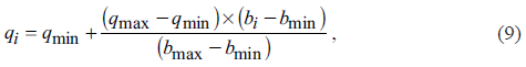
where q i . represents the normalized data, b i . is the measured coordinate values, while b min .and b max represents the minimum and maximum value of the measured coordinates with q max and q min values set at 1 and -1, respectively.
Statistical Resampling Technique
Generalisation is a generic operational procedure use to assess the efficiency of developed mathematical and statistical models. In common terms, generalisation is the ability of a model to correctly learn the significant parameters of a prediction function (training set) and predict well on yet unseen data (testing data) (Urolagin, 2011). The general way adopted in the majority of research works relating to coordinate transformation for assessing the generalization capability of a model is by using the hold-out cross-validation technique (Gullu, 2010; Lin and Wang, 2006; Mihalache, 2012; Tierra et al., 2008, 2009; Tierra and Romero, 2014; Turgut, 2010; Gullu et al., 2011; Yilmaz and Gullu, 2012; Zaletnyik, 2004; Konakoglu and Gökalp, 2016; Konakoglu et al., 2016; ElSayed and Ali, 2016; Ziggah et al., 2016; Ziggah et al., 2017a). However, as stated earlier (introductory section), the hold-out cross-validation method has some deficiencies to be surmounted. Therefore, a solution to the enumerated problems has led to the usage of K-fold cross-validation (KCV) as an alternative way to estimate out-of-sample accuracy.
The KCV is a procedure that employs the entire dataset as training and testing sets (Bengio and Grandvalet, 2004). By virtue of using a combination of more tests, a stable estimate of the model error could be achieved (Reitermanová, 2010). This is because each point in the entire dataset will be in a test set just once, and will be in the training set the number of folds. Hence, for KCV approach how the entire dataset is divided is less of a concern as compared with the hold-out approach.
In the KCV method, a K-fold partition of the entire dataset is first carried out. Here, the dataset M is separated into K disjoint blocks of approximately equal size as the target data such that
 (Konaté et al., 2015).
Subsequently, for each K trials of cross validation the union of K-1 folds is used as training data for model development while the remaining part is used as the testing data for the resulting model validation (Stone, 1974). In this study, the K-1 disjoint set was used to train the RBFNN as well as to determine the transformation parameters for the Bursa-Wolf model. The remaining subset acting as the test data was used to validate the results produced by RBFNN and Bursa-Wolf model, respectively. This K-fold methodology was applied to the 19 co-located points (Table 1) located in the Golden Triangle (Fig. 1) from the Land Administration Project.
Table 1 Co-located point in the Ghana geodetic reference network showing K-fold partition (subset 1, 2, 3 and 4). The WGS84 coordinates for longitude, latitude and ellipsoid height are represented as WGS LONG, WGS LAT in decimal degree unit and WGS HGHT in meters. WAR LONG, WAR LAT, WAR HGHT are the corresponding coordinates on the War Office 1926 ellipsoid.
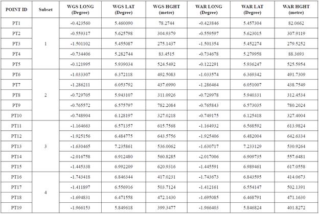
In practice, the 19 common points was divided into four disjoint subsets (four-fold) as shown in Table 1 as subset 1, 2, 3 and 4 respectively. It can be seen from Table 1 that subsets 1 to 3 comprised of five common points, while subset 4 consisted of four data points. After dividing the entire dataset into four-folds (Table 1), four models were then built using each subset. In this process, for each trial one part of the data is kept for testing and the remaining parts for training as shown in Table 2. That is, in the present study, there are three parts for training and one part for testing at each step. This is evident from Table 2 where it can be seen that the first row in subset 1 has been singled out for testing, while the second to fourth rows data are used for the training. In subset 2, the second row was set for testing while the first, third and fourth rows were used for training. This same procedure was continued for subsets 3 and 4 as indicated in Table 2, respectively.
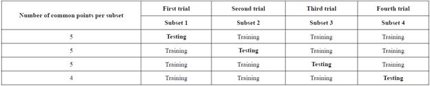
A critical study of Table 2 shows that there is no overlap between the subsets and no overlap between the testing data. However, there is significant overlap of the training parts. This implies that in the K-fold cross-validation system each data subset is passed exactly once as a test sample. In the present context, RBFNN and Bursa-Wolf model was trained and tested in four trials with four coordinate transformation models being developed simultaneously. Therefore, the average accuracy produced over all the four disjoint subsets served as a better indicator for the out-of-sample rotation performance of the RBFNN and the Bursa-Wolf model in the study area. It should be known here that the same subset data applied in the RBFNN was used for the Bursa-wolf model.
Statistical Performance Metrics
The usefulness of any applied mathematical or statistical model depends on how close their predicted outcomes fit well with the observed data. By applying statistical quantitative methods, an objective evaluation of the quality of the results produced by the model could be done. In lieu of this, the following statistical performance metric (PM) tools were employed.
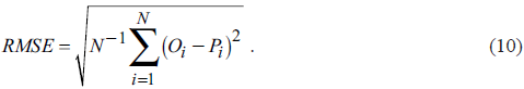
(i) Root Mean Square Error
The root mean square error (RMSE) is a type of dimensioned error statistic that is always non-negative and incorporates the concept of bias and standard deviation. It is used to quantify the degree of dispersion of model predictions to observed data in a system. Ideally, an optimum model performance should have a RMSE value of zero. However, in practice, the RMSE could vary from zero to infinity subject to the units of the forecasted variable. Equation 10 was applied in the RMSE estimation expressed as
(ii) RMSE Horizontal Positional Residual
The RMSE horizontal positional residual (RMSEHE) technique was used to determine the total uncertainties in the integrated data set used. The RMSEHE (Paredes-Hernández, 2013) is given by Equation 11 as follows:
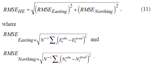
The RMSEEasting and RMSENorthing is the RMSE in Easting and Northing coordinates. E i obs , Ep red i , N i obs and N i pred signify the observed and predicted Easting and Northing coordinates.
Easting Northing.
(iii) Standard Deviation
The standard deviation (SD) was computed to assess the precision of the transformed coordinates produced by the model. It is calculated in Equation 12 as
Here, e represent the deviations between the observed and predicted data and ē is the average of the deviations.
(iv) Horizontal Positional Residual
The Horizontal positional residual (HE) was used to ascertain the horizontal accuracy associated by integrating the transformed horizontal coordinates for each position. The HE could be represented by Equation 13 as
where (EO, NO) are the observed coordinates and (EP, NP) are the transformed coordinates given by the model.
Transformation Parameters Determined and RBFNN Model Developed
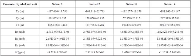
The application of the similarity transformation model of Bursa-Wolf requires the determination of seven unknown coordinate transformation parameters. This study deduced these parameters from a sequence of 19 common points in WGS84 and War Office 1926 reference frames. It was however observed that the number of available common points will generate more equations than the seven unknown transformation parameters needed. This will as a result, create an over-determined system of linear equations that require a more pragmatic technique to find solutions to them. To overcome this problem, the total least squares adjustment technique described in Sect. 3.2 was applied to the Bursa-Wolf model for the calculation of the transformation parameters and their standard deviations. It must be known that the training and testing data for each subset (Table 2) was used to determine the transformation parameters and checking model performance. These determined parameters involved three translation vectors (Tx, Ty, Tz), three rotational parameters (Rx, Ry, Rz), and one scale factor (Sf) as shown in Table 3. For the purpose of this study and to provide adequate objective comparison of the Bursa-wolf model to the RBFNN, the transformation parameters were determined for each subset. Table 3 presents the transformation parameters, with the addition of their standard deviations for each subset.
Table 3 Computed transformation parameters for the Bursa-Wolf transformation model for on each partition
The proposed RBFNN model developed for transforming coordinates from WGS84 to War Office 1926 reference frame comprise of three layers: input layer, hidden layer and output layer. In the RBFNN model development process, the same K-fold split data (Tables 1 and 2) set used for the Bursa-Wolf was employed. The supervised training technique was adopted in the RBFNN model formulation. The data was first normalised into the range of [-1, 1] using Equation 9. This was necessary in order to bring the entire data onto a common scale interval thereby achieving equal variations among the datasets. In this study, the RBFNN structure consists of two inputs, one hidden layer using Gaussian function as the non-linear transfer function, and an output layer having linear transfer function. The data for each subset (see Tables 1 and 2) was trained and tested by the RBFNN.
To do that, several input and output data scenarios were tested with the objective of selecting the one that produced better transformed coordinate values.
Here, (X, Y, Z)WGS84 and (X, Y, Z)WAR was first applied as the input and output data, respectively. Secondly, (φ,λ, h)WGS84 and (φ,λ, h)WAR was used as input and output. Finally, (φ,λ)WGS84 was used as input with (φ,λ)WAR as the output. The coordinates used here are defined in Table 1. The input-output scenario was made possible due to the non-parametric capability of the RBFNN. Thus, the RBFNN does not require a mathematical function to describe the input-output relationship among the variables. It was observed that the third scenario yielded more satisfactory results.
In deciding the optimal RBFNN for each subset (see Tables 1 and 2), the MSE (Equation 7) of all the trained models were examined at each stage of training and testing. Here, the MSE was serving as the optimality criterion to facilitate in choosing the best RBFNN structure for each trained subset suitable for coordinate transformation from WGS84 to Ghana War Office 1926. Therefore, the trained network that produced the lowest MSE from the testing dataset was chosen as the best RBFNN scheme.
After several trials, the optimum RBFNN scheme for subsets 1, 2 and 3 (Tables 1 and 2) was [2-14-2], while subset 4 had [2-15-2], respectively. The interpretation here is that, two inputs (φ,λ)WGS84, one hidden layer of14 neurons and two outputs (φ,λ)WAR, was achieved for subsets 1, 2 and 3 whereas, subset 4 differed only by the number of hidden neurons (15) as its optimal number. The results produced by these optimum RBFNN models were then projected onto the Transverse Mercator 10 NW to get the projected grid coordinates. This was done by using equations from Ayer (2008). For the case of the Bursa-Wolf model, the transformed rectangular coordinates was first converted into geodetic coordinates using Bowring Inverse Equation (Bowring, 1976) and then projected onto the Transverse Mercator. These projections were necessary because Ghana utilises the 2D projected grid coordinate system (Easting, Northing) for its surveying and mapping related activities.
K-fold Cross-Validation Analysis
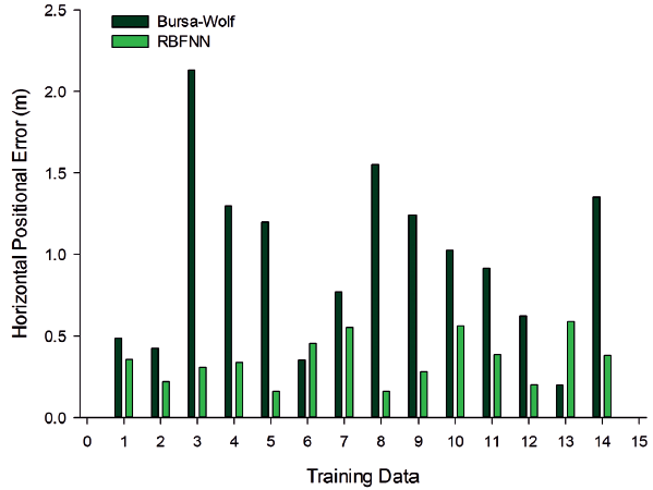
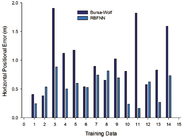
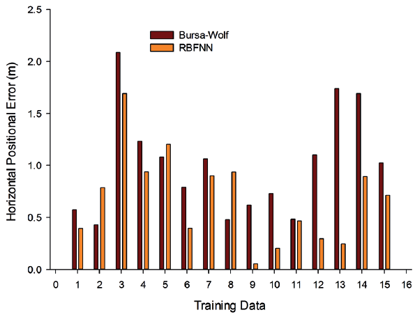
The K-fold cross-validation technique enables the modeller and the user to have an honest assessment of the models predictive performance. The objective here is to test the potential of RBFNN via KCV for the first time in coordinate transformation under data-insufficient situation in Ghana geodetic reference network. In order to evaluate the extent at which the RBFNN and Bursa-Wolf model transformed coordinates deviate from the measured, horizontal positional residuals using Eq. (13) were estimated and evaluated. The essence is to know the practical application of the Bursa-Wolf and RBFNN transformed coordinates. The various positional errors determined at the training and testing stages for all the four-folds are shown in Figures 3 to 10, respectively.
With reference to Figures 3, 4, 5 and 6, it is known that the respective transformed training coordinates from the RBFNN model demonstrated low bias in the training data than the Bursa-Wolf model. This means that the RBFNN transformed outputs do not differ greatly from the measured (target) training data and thus was able to learn the training data in a more effective manner due to its adaptive computational capabilities compared with the parametric method of the Bursa-Wolf model. This phenomenon was observed in all the four-folds of the training data as shown in Figures 3, 4, 5 and 6, respectively.
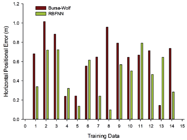
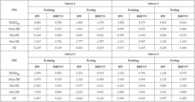
Figures 7, 8, 9 and 10 display how well the Bursa-Wolf and RBFNN models generalised on the testing data for the four-folds. It is acceptable that the strength of a model lies in its ability to give a least prediction error when unseen data is introduced into the model. A visual inspection in Figures 7, 8, 9 and 10 clearly exposed the strength of RBFNN generalisation over the Bursa-Wolf model in terms of horizontal accuracy. Moreover, Figures 7, 8, 9 and 10 suggest that encouraging horizontal coordinates were produced by the RBFNN model. Furthermore, these assertions are buttressed by the interpretation of the quantitative estimations of the horizontal positional accuracy assessment for the training and testing set as presented in Table 4.
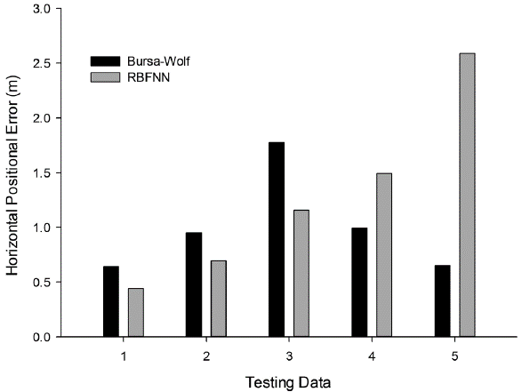
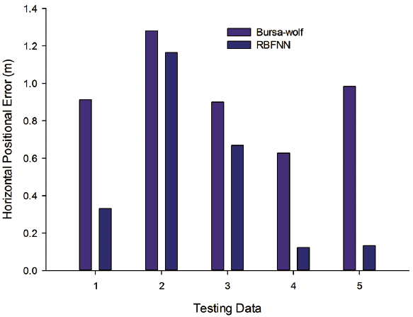
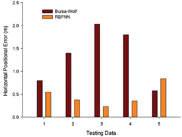
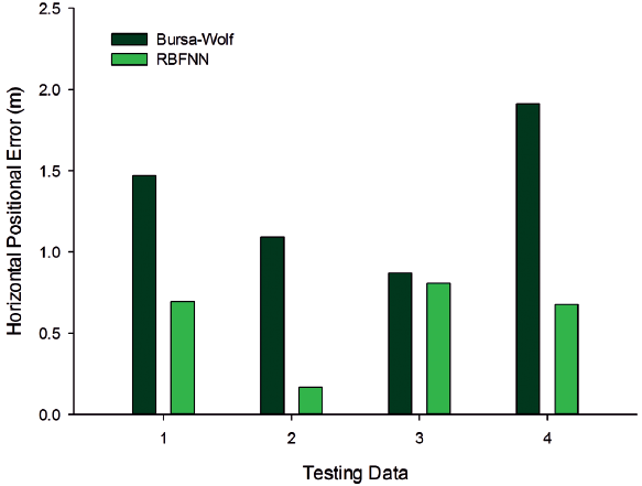
Table 4 Statistics of the total horizontal residual assessment for the training and testing data across the 4-folds (unit: metre)
It is well understood that to evaluate the overall performance of a model via KCV technique, there is the need to find the average across the K-folds 'optimal' models error estimates as quantified by the performance metrics (Jung and Hu, 2015). That is, find the average of each performance metric results presented in Table 4 across the entire four-fold. Hence, the four-fold cross validation technique average performance based on the statistical analytical tools applied to the Bursa-Wolf and RBFNN transformed coordinates is given in Table 5.
Table 5 Statistics of the overall average horizontal positional errors for Bursa-Wolf (BW) and RBFNN across the 4-folds (unit: metre)
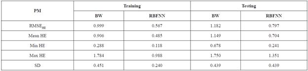
As can be seen from the descriptive statistics in Table 5, it is noticeable that the RBFNN model performed better than the Bursa-Wolf model. The RMSEHE test results (Table 5) indicate that the RBFNN model had the least total horizontal dispersion of 0.797 m, while 1.1820 m was achieved by the Bursa-Wolf model. These RMSEHE calculated values describe the total uncertainties exhibited in the entire integrated horizontal coordinates. On account of the Mean HE test results (Table 5), it could be stated that when the RBFNN model is applied in the study area, a horizontal positional error in average of 0.704 m would be produced as compared with 1.149 m by the Bursa-Wolf model. These mean HE values denote the achievable average horizontal positional error for Bursa-Wolf and RBFNN models, respectively. The maximum and minimum HEs (Table 5) suggest the interval at which the error produced by Bursa-Wolf and RBFNN varies in the study area. Observation from Table 5 shows that the RBFNN achieved the best minimum (0.241 m) and maximum (1.351 m) HE test results. Thus, the RBFNN has the capability of producing satisfactory transformation results in the Ghana geodetic reference network (Golden Triangle) than the Bursa-Wolf model. From the SD computed values (Table 5), it could be seen that similar transformation precision was produced across the four-folds by RBFNN and Bursa-Wolf model, respectively.
Consistent with the results in Table 5, it is clear that for the study area the RBFNN approach is superior to the Bursa-Wolf model. The strength of the RBFNN could be attributed to its non-parametric properties whereby it has the capability to adapt to the dataset without a priori knowledge of the underlying functional relationship describing the input and output dataset. From these results, it can be stated that the application of RBFNN via KCV approach for coordinate transformation in Ghana geodetic reference network has been duly demonstrated. Furthermore, the transformation errors produced in this study could possibly be attributed to the coordinates related to the Ghana local geodetic reference system (Accra datum) than the global WGS84 data. This is because with all the attendant problems of local geodetic networks as indicated by several authors (see e.g. Poku-Gyamfi, 2009; Varga et al., 2017 and references therein), the coordinates of the Accra datum lacks homogeneity. It is therefore logical to state that these distortions inherent in the network might have contributed to the level of accuracy achieved in this study. Nonetheless, it is suggested here that the obtained results produced could still be used in Ghana for low-order survey works such as data collection for geographic information system geodatabase generation, reconnaissance survey, small scale topographic surveys and for land information system works. This assertion was based on the maximum allowable horizontal positional error tolerance of ± 0.9144 m set by the Ghana Survey and Mapping of Lands Commission for cadastral applications and plan production in Ghana (Yakubu and Kumi-Boateng, 2015).
Concluding remarks
The hold-out cross-validation procedure has been widely adopted to assess the performance of the coordinate transformation methods. However, studies have shown that the KCV offers some advantages over the holdout approach. Therefore, the main contribution of this study is to apply and demonstrate the potential and applicability of the RBFNN via KCV technique on the LAP sparse dataset in Ghana geodetic reference network. The obtained RBFNN results were compared with the Bursa-Wolf model. The findings revealed significantly that improper split of the sparse dataset for the Ghana geodetic reference network into single train-test experimentation could produce misleading results that is totally dependent on how the data was partitioned and the split set selected. These are evident from the four-fold results produced by Bursa-Wolf and RBFNN where if a particular split fold is chosen for the case of hold-out cross-validation would give a misrepresentation of the models capability. Hence, it has been demonstrated in this study that for proper assessment of model predictive performance especially in sparse dataset situation, the KCV offers a better solution.
The conclusion made from the overall statistical analyses was that, for Ghana geodetic reference network the RBFNN has the potential and strength to account for the uncertainties in the data related to the different data (War Office 1926 and WGS84) more effectively than the Bursa-Wolf model. The result suggests that the RBFNN will be more applicable to low-order accuracy surveys. This is because the RBFNN achieved maximum horizontal positional error was more than the ± 0.9114 m tolerance set by the Ghana Survey and Mapping Division of Lands Commission for cadastral applications.