


 English (pdf)
 Article in xml format
 Article references
 Send this article by e-mail
 Cited by SciELO
  Cited by Google
  Similars in
SciELO
Similars in
SciELO  Similars in Google
 Permalink
Introduction
Wedge failure is a kinematically controlled mechanism of failure, in which the relative position of joint and slope planes controls the stability. This mechanism is widespread in both highway and open pit excavations. Limit equilibrium (LE) is a suitable approach to calculate the stability of potentially unstable rock wedges. LE provides a closed form solution to well-defined wedge geometry to calculate the factor of safety, which is convenient when performing a reliability assessment.
Although LE provides a practical solution to the problem of wedge stability, the inputs determination is not straightforward, since rock mass is a heterogeneous material, in which properties change from point to point. This variability introduces uncertainty to the model. Moreover, in mining projects, new and variable information is available, as the exploitation progresses. Considering that the information is variable, different results are obtained at different stages of the project operation. Hence, in this sort of projects, the decision-making process should be a dynamic task, assisted by geotechnical models able to incorporate new information and to update the results.
There are several alternatives to cope with uncertainty. For engineers, the most popular alternative is the purely probabilistic approach, with some documented drawbacks; the actual meaning of the probability of failure and the need for information, which is not available in most geotechnical projects (Oberguggenberger, 2012). Therefore, alternative and more flexible approaches have been developed to deal with uncertainty under limited information (Couso, Dubois, & Sánchez, 2014).
These alternative approaches are based on interval analysis and correspond to imprecise probabilities techniques. Among these techniques, the random sets theory (RST) is a suitable tool to perform reliability assessment in geotechnical problems, including the input parameters as intervals (Oberguggenberger, 2012). RST, also, offers a systematic way to combine different pieces of evidence and adjust the reliability assessment results, at different stages of the project. This combination is performed according to the mixing (or averaging) of evidence rule, under the evidence theory framework (Sentz & Ferson, 2002).
The concept of RST as presented in this document corresponds to the interpretation of Dempster (1967) of the Belief function as the lower probabilities induced by a multivalued mapping. According to this approach, a multivalued mapping from a probability distribution generates a set-valued random variable, that is a more complex object than the standard random variable. The original work developed by Dempster was reinterpreted and generalized by Shafer (1976) to develop their evidence theory, which building block is the probability distribution on the power set of a finite set (Couso et al., 2014), i.e., a random set.
Although before Shafer's (1976) work there were no practical applications of RST, since 1990's there has been a geometrical growth on the number DST applications (Beynon, Curry, & Morgan, 2000). Some examples of the most recent publications on the topic include measuring uncertainty in big data (Dutta, 2018), multisensor-based activity recognition in smart homes (Al Machot, Mayr, & Ranasinghe, 2018), skin diseases (Khairina, Hatta, Rustam, & Maharani, 2018), cancer detection (Kim et al., 2018), fault in power transformers (Kari et al., 2018), heritage evaluation (Liu, Zhao, & Yang, 2018), thermal plants monitoring (Moradi, Chaibakhsh, & Ramezani, 2018) and chemical risk assessment (Rathman, Yang, & Zhou, 2018). These are just a few examples to illustrate how relevant is this approach to handle decision making under uncertainty.
The number of publications on the geotechnical is not comparable to other fields like AI or medicine. However, there is a growing interest of the geotechnical community in involving the evidence theory in the decision-making process. The first application attempted to predict the rock mass response around a tunnel excavation (Tonon, Mammino, & Bernardini, 1996). Likewise, Tonon, & Bernardini (1999) pursued the problem of optimization of the lining using RST and fuzzy sets. Subsequently, Tonon, Bernardini, & Mammino (2000) presented an application to compute rock mass parameters (RMR) of rock masses. Moreover, Tonon, Bernardini, & Mammino (2000b) performed plane failure analysis and tunnel lining design with simple explicit models using RST and Monte Carlo simulation. They also showed the advantages of using the concept of strictly monotonic functions to reduce the number of computations, which reduces the computational cost of this approach.
A framework to develop a reliability assessment of geotechnical problems by finite element methods and RST was developed by Peschl (2004). This work presents a comprehensive methodology to perform reliability assessment, in which inputs are expressed as random sets, leading to a bounded probability function for the finite element model results, e.g., displacements. This application was named random sets finite element method, RS FEM. Subsequently, related documents have been published with applications of the RS FEM (Schweiger & Peschl, 2005; H. F. Schweiger & Peschl, 2004, 2005). Besides, this method has been applied to the analysis of tunnel excavations (Nasekhian & Schweiger, 2011).
Klapperich, Rafig, & Wu, (2012) and, Shen, & Abbas (2013) combined RST with the distinct element method to assess the stability of rock slopes. In this case, the deterministic reference model is run using the discrete element software UDEC (Cundall, 1980), according to the realizations defined by the combinations of the input random sets. With the results, cumulative probability distributions were computed.
In this context, this paper presents the RST as an alternative to deal with uncertainty, under limited information. The approach is applied to evaluate the stability of wedges in a sandstone quarry located in Une, Cundinamarca, Colombia, that has been under operation for 20 years. Thus, as new information is available, the analysis is updated.
The first part of the paper presents a description of the wedge LE model selected. Subsequently, a brief description of RST is offered, along with an approach to perform sensitivity analysis and the combination of evidence. A practical example at a sandstone mine in Une, Cundinamarca, Colombia is presented using this approach. Lastly, based on the results, conclusions are drawn.
This research aims at contributing to the process of rock slope stability analysis by considering one mechanism of failure (wedge failure). Nevertheless, the design of a rock slope is a very complex task, in which several mechanisms of failure and triggering factors are involved. Hence, additional work on random sets applied to rock slope stability is required.
Wedge stability model
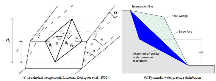
The geometry of the wedge analyzed in this project is defined by four planes; two discontinuities and two free surfaces (slope face and upper slope) as shown in Fig. 1(a). Tension cracks are not explicitly considered. The stability assessment of wedges implies the formulation of equilibrium of forces in a three-dimensional space. This problem has been solved by using stereographic projections (Goodman & Taylor, 1966; Hoek, Bray, & Boyd, 1973; and Goodman, 1995).
However, when a reliability assessment is performed, a closed-form solution is more suitable because several realizations of the model should be computed. Low (1979) developed a closed-form equation without using graphical assistance; subsequently, Einstein & Low (1992) extended this solution considering an inclined upper slope. The approach has been applied to perform wedge failure reliability assessment (Einstein & Low, 1992; Jimenez-Rodriguez, Sitar, & Chacón, 2006; Low, 1997; Low & Einstein, 2013). The reliability of wedges has also been studied considering multiple correlated failure modes (Li & Zhou, 2009; Li et al. 2009) and knowledge-based clustered partitioning approach (Lee et al., 2012).
The solution proposed by Low (1979) was selected to account for the uncertainty in this work since it is convenient to perform several realizations of the model. A brief description of this proposal is given below.
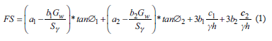
The model can analyze four modes of failure in this sort of wedges: failure along the intersection of both joint planes, failure along either joint plane 1 or plane 2 (the planes order selection is arbitrary), and lifting failure. The factor of safety (FS) for this mode can be calculated according to Eq. (1) (Low, 1997):
This equation is valid only when:
In which:
Ø t and Ø 2 are the friction angles of planes 1 and 2, respectively
c 1 and c 2 correspond to the cohesion of planes 1 and 2, respectively
G W is the water pressure coefficient of a pyramidal distribution, as shown in Fig. 1(b)
A is the slope face inclination
h is the slope height, and H b is the total height, including the upper slope with inclination Q
α 1 , α 2 , b 1 and b 2 are geometric coefficients; a function of the following angles (for a detailed description see (Low, 1997))
β 1 is the horizontal angle between the strike line of plane 1 and the line of intersection between the upper ground surface and the slope face. Idem for
β 2 in plane 2 (Jimenez-Rodriguez, Sitar & Chacon, 2006)
δ 1 and δ 2 are the dip angle of plane 1 and 2 respectively
ε is the inclination (plunge) of the line of intersection between planes
s v is the specific weight of the rock
Random Sets Theory
Definition
To define a random set, suppose that M observations were made of a parameter u Є U, each of which resulted in an imprecise (non-specific) measurement given by a set A of values. Let c. denote the number of occurrences of the set A. Є U, and φ(U) the set of subsets of U. A frequency function m can be defined such that (F. Tonon et al., 2000a):
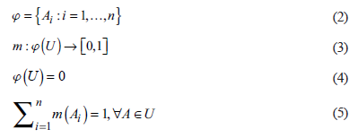
φ is called the support of the random set, the subsets A. are the focal elements and m is the basic probability assignment. A pair (φ, m) defines a random set. Each set, A. Є p, contains possible values of the variable, u, and m(A) is the probability associated with A (H. F. F. Schweiger & Peschl, 2005).
When working in the space of real numbers, the support of the random set, φ, is given by intervals, with their corresponding probability assignment. In this paper, the uncertain parameters are considered as intervals (rock mechanical properties and joints geometry), without any specific information related to the distribution or variation between the extremes of the interval, along with the probability assignment.
Accordingly, if the focal element A
i
. is a closed interval of real numbers expressed as:
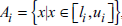 , thelower (F*)and the upper cumulative probability distribution functions (probability function) can be computed as follows (Peschl, 2004):
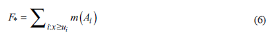
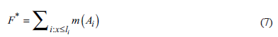
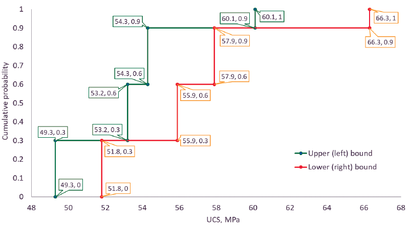
In other words, to obtain the left envelope (upper bound), the distribution function of each interval in the calculation matrix is assumed to be concentrated at the lower bound of each focal element. On the other hand, for the right envelope (lower bound) the probability mass for each interval is assumed to be concentrated at the upper bound of the interval (Schweiger & Peschl, 2005). The bounded distribution function defined by the upper and lower bounds is referred to as BDF.
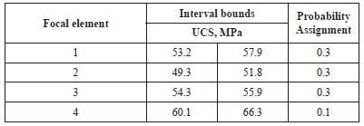
The following example illustrates the concept of a random set. Let assume a layer of sandstone, from which four block samples were taken. From each block, two cores were taken and tested to measure the uniaxial compressive strength, UCS. Due to local regulations, two different laboratories tested the samples. However, design engineers have more confidence in the results from laboratory 1, because it provides certified testing services, while the second does not. Table 1 summarizes the test results.
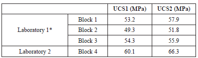
Based on their experience and judgment, the design team defined a random set for the sandstone uniaxial compressive strength, UCS, like the one shown in Table 2. Such a random set has four focal elements, A, defined by the strength intervals resulting from each sample. The set of these intervals forms the support of the random set. Moreover, each focal element has a probability attached, i.e., the probability assignment, m. The probability was assigned based on the reliance of engineers on each laboratory. In this example, the results from each block define the random set. However, the selection of the focal elements and probability assignments should be the result of sound engineering judgment.
With the random set, the bounded probability distribution function (BDF) for the UCS of the sandstone can be constructed according to Eqs. 6 and 7. Fig. 2 shows the BDF, where the original focal elements bounds are explicitly marked. Here, the orange and green lines represent the lower (right) and upper (left) bounds of the UCS BDF, respectively.
Function of random sets
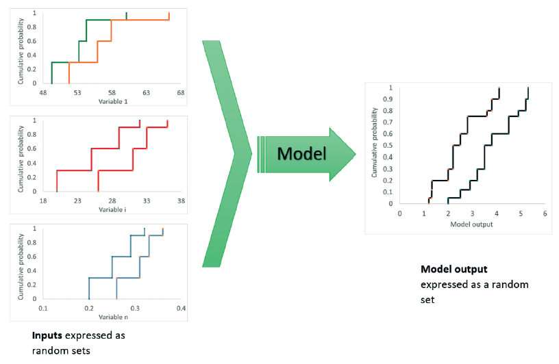
Once the random sets of input parameters are defined, three main tasks should be performed to compute a bounded distribution function (BDF) of the assessed system. Firstly, the image (output) of the input random sets through a function f has to be established. Subsequently, a probability assignment should be assigned to the computed image. Finally, a bounded cumulative distribution function of the output is calculated, according to Eqs. 6 and 7. Below, a brief description of these steps is presented.
Assume a random set (R, p), which is the image of (T, m) through a function f. The set (R, p) is described as follows (Schweiger & Peschl, 2005):
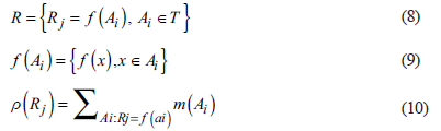
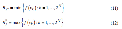
Assuming that the function f(A i ) is continuous in all A i . Є T, and no extreme points exist in this region, except at the vertices, the vertex method applies to calculate the image (R, p) of the input random set through the function f (Schweiger & Peschl, 2005). Assume each focal element A i . is an N-dimensional box, whose 2 N vertices are indicated as v k , k = 1,... ,2N. If the vertex method applies then, the lower and upper bounds R j , and R* on each element R. G R will be located at one of the vertices (Schweiger & Peschl, 2005).
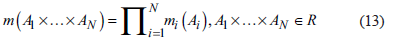
As for the probability assignment of the output, if A 1 ,, A n are sets on X 1 x ... x X n , respectively, and x 1 , ..., x N are random independent sets, then the joint probability assignment is measured by:
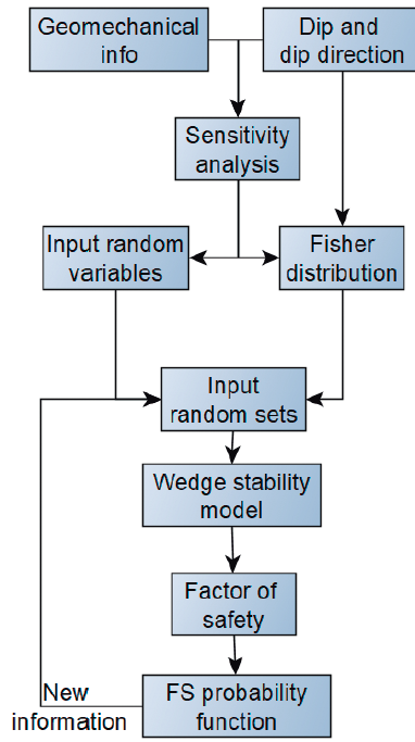
The bottom line is that RST allows involving the inputs into the problem as random sets, through a function or a model (in this case, the wedge slope factor of safety function, Eq. (1)) to obtain a bounded distribution function (BDF) of the response. A diagram of that process is depicted in Fig. 3.
A complete description of the theoretical background of RST and its applications can be found in Bernardini and Tonon (2010).
Combination of random sets
According to the concepts just presented, RST offers an alternative to performing reliability assessment concerning intervals and probabilities, when limited information is available. This approach also offers an alternative to systematically include new information to adjust or update the cumulative probability functions.
The problem of combining several pieces of information is addressed by Dempster-Shafer Theory of evidence (DST) (Shafer, 1976) and is suitable to consider the limited information when it has both epistemic and aleatory uncertainty (Sentz & Ferson, 2002), even when expert opinion is involved (Torkzadeh-Mahani et al., 2018). This is the case that is assessed in this paper, which deals with information from different sources, at different stages of the project (pieces of information).
The primary goal of aggregation or combination of information is simplifying or summarizing information that comes from several sources into one set of evidence (Sentz & Ferson, 2002). In a DST framework, each piece of information is expressed as a random set and then combined with other pieces of information by redefining the focal elements and allocating different probability assignments. There are several rules to combine information, which differentiate on the way to allocate the probability assignment. For a detailed description of evidence combination rules under DST see Sentz & Ferson (2002) and some examples applied to engineering problems can be found in Zargar et al. (2012)
For this paper, the mixing or averaging method was selected, since this technique generalizes the averaging operation frequently used for probability distributions, which is regarded as a natural method of aggregating probability distributions. Hence, it is reasonable to consider this approach to average random sets. This combination rule has been applied to geotechnical problems including the finite elements method (Peschl, 2004). A brief description of this rule is given below.
Let suppose a rock slope excavated in different stages, before getting the final configuration. At each stage, information on joints geometry and joint mechanical properties are collected. Therefore, the information of any parameter Z is described by a random set (e.g., the friction angles are described by intervals with their corresponding probability assignment). Suppose there are n stages, so the variable is described by n alternative random sets, each one corresponding to an independent source of information. The method modifies the probability assignments, m,, as follows:
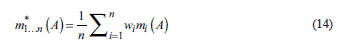
In which w. are weights assigned according to the reliability of the sources and m 1 * is the probability assigned to the combined focal element.
Sensitivity Analysis
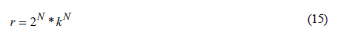
To compute the distribution functions, selection of the most influencing variables is required. These variables are modeled as random sets, while the others as deterministic, which is a crucial step since the number of random sets defines the number of realizations of the model. For instance, if there are N random variables, each one with k focal elements, the number r of realizations of the model would be:
The sensitivity analysis also allows knowing the variation of the response of the model with the different variables. With this information, the proper combination of input variables can be defined at each N-dimensional box to define the maximum and minimum results of the model, without computing every combination at that box. Hence, the number of computations reduces to:

To perform reliability assessment in geotechnical problems applying the concept of RST, Peschl (2004) adopted a methodology based on a central difference approach, in which a sensitivity ratio (nSR) is computed (EPA, 2002).
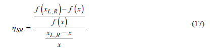
Where x is the reference value, X l,R and f(x) and f(x LR ) are the outputs of the functions at those points. The sensitivity ratio is local, varying x L a small amount from the reference value, and general changing x R across the whole range. Therefore, if there are N variables, n SR should be computed 4N+1 times.
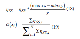
The sensitivity ratio is normalized according to Eq. (18), then a total relative sensitivity index (α(x i )) is computed for each input variable. The last latter index varies between 0 and 1 and measures the influence of a given variable in the function. The higher α(x i .), the more the influence of the variable in the output.
The sensitivity analysis also provides a few realizations of the model, within a representative interval. Hence, it is possible establishing the local variation of the function for each input variable. In other words, the sensitivity analysis allows to establish if the model is increasing or decreasing concerning a variable, within an interval, which reduces the number of computations to define the upper and lower bounds for combinations of focal elements.
Example Analysis
The concepts just presented related to wedge failure and RST were applied to a sandstone mine situated in Une, Cundinamarca, Colombia. This mine is in a sedimentary rock mass, formed mainly by alternating layers of sandstone and shales. The mine has been operated since 1990ies until nowadays.
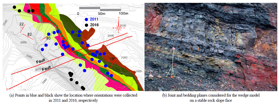
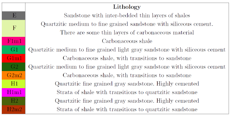
Fig. 4(a) shows the surface geology of the mine and the points where planes orientation were collected in 2011 (blue) and 2016 (black). The descriptions of the lithologies is included in Fig. 5. Besides, Fig. 4(b) presents a picture of the rock mass, in which the joint and bedding planes are shown on a stable rock slope.
During its operation, a detailed geological and geotechnical monitoring has been carried out at the mine slopes. As a result, a complete data set on joints dip and dip direction is available. Besides, a few results of mechanical tests like unconfined compression strength (UCS) and shear behavior along discontinuities were collected. The first information was collected in 1997 when the operation started. Then in 2011 a detailed geotechnical assessment to update the mine design was carried out, which included a back-calculation of a rock slope failure reported in 2000. Finally, as part of a research project, new information was collected in 2016.
Table 3 shows the results of strength parameters along discontinuities in shale layers. In regarding these results, some values of cohesion were measured in the laboratory. As for the samples tested in 2016, the cohesion is apparent and associated with the texture of the joint, rather than any filling within the joint. No information is provided related to cohesion from samples collected in 1997 and 2011.
Table 3 Mechanical properties measured on rock joints
| Peak | Residual | Peak | Residual | Unit | ||
|---|---|---|---|---|---|---|
| Year | Sample | cohesion | Cohesion | friction | friction | weight |
| (kPa) | (kPa) | angle (°) | angle (°) | (kN/m3) | ||
| 1997 | 1 | 32.5 | 2.9 | 22.5 | 22.0 | 26.2 |
| 8.2 | - | 29.5 | - | - | ||
| 2 | - | - | 26.3 | 17.6 | 23.6 | |
| 7.8 | - | 23.6 | - | - | ||
| 2011 | 1* | - | 18.0 | - | 18.0 | 26.0 |
| - | 6.0 | - | 20.0 | - | ||
| 1 | 87.3 | 39.6 | 29.2 | 23.9 | 24.3 | |
| 2 | 89.2 | 25.5 | 34.8 | 32.8 | 23.6 | |
| 3 | 17.6 | - | 40.4 | 36.6 | 23.9 | |
| 2016 | 1 | 48.0 | - | 31.8 | - | 24.2 |
| 2 | 69.0 | - | 22.0 | - | 24.8 | |
| 3 | 97.0 | - | 18.5 | - | 24.8 |
*From the back analysis
Table 4 summarizes joint planes dip and dip direction and slope geometry. Sources of information listed in Tables 3 and 4 are assumed to be independent. In this case, this assumption is reasonable, since the information was collected at different times, by different groups of people and with different tools.
Table 4 Joint plane and slope mean parameters
| Plane | Dip direction (°) | Dip (°) | Height (m) |
|---|---|---|---|
| Bedding | 306 | 26 | - |
| Joint set 1 | 57 | 82 | - |
| Slope | 329 | 70 | 25 |
Once the input information is defined, the steps followed to perform an update the probability of failure is depicted in Fig. 6. At this point, it is important to highlight that two types of information can be distinguished. Firstly, there are just ten results on strength parameters of the rock masses, collected for 20 years, while there are 967 poles measured during the same period.
The wedge failure model selected for this paper has been developed for wedges delimited by two joint sets, the slope face and the upper slope. Based on this information, the model has 13 variables, including geomechanical and geometrical variables.
Results
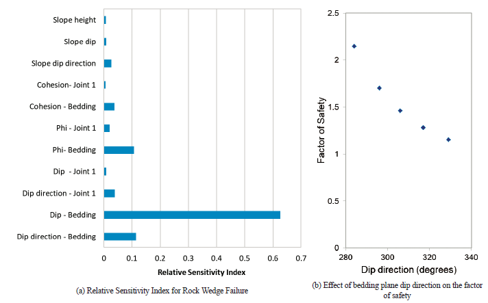
With the slope model and input variables fully established, the next step is to define the most influencing variables on the wedge response, which is accomplished by the sensitivity analysis described in section 3.3. Therefore, the factor of safety was computed with Eq. (1), and the weighted sensitivity indexes, a, were computed and plotted in Fig. 7(a). The three variables with the highest a were selected as random sets and the rest as deterministic. Hence, the random sets are the dip and dip direction of the bedding, as well as, its friction angle.
Next step is defining the input random sets. In regarding friction angle, assumptions are required because few data are available. Hence, for the information collected in 1997 and 2011, the random sets were defined considering that the actual value of the friction lies somewhere between the peak and the residual friction. These values are conservative compared with the focal elements selected for 2016, in which only peak friction angle was considered, as there are no residual values reported. Table 5 shows the selected random sets.
Table 5 Input random sets on bedding plane friction angle
| Year | Bedding plane friction angle (°) | ||
| Lower | Upper | PA* | |
| 1997 | 22.0 | 22.5 | 0.33 |
| 22.0 | 26.3 | 0.33 | |
| 17.5 | 23.6 | 0.34 | |
| 2011 | 23.9 | 29.2 | 0.33 |
| 32.8 | 34.8 | 0.33 | |
| 36.6 | 40.4 | 0.34 | |
| 2016 | 22.0 | 31.8 | 0.50 |
| 18.5 | 22.0 | 0.50 | |
*Probability Assignment
Conversely, vector information on joints orientation and dip were pre-processed to be expressed as intervals. Considering that these data are vectors, they were assumed to fit a Fisher distribution. This distribution assumes that a population of poles is distributed around a true orientation (Fisher, 1953). Then, angles for confidence regions of 40% and 90% around the true orientation were calculated based on the measured orientations. Afterward, new interval bounds were defined as follows (see Table 6):
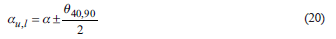
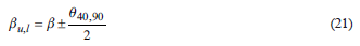
Table 6 Input random sets on bedding dip and dip direction
| Bedding | |||||||
|---|---|---|---|---|---|---|---|
| Year | ID | Dip direction (°) | Dip (°) | ||||
| Lower | Upper | PA | Lower | Upper | PA | ||
| 313 | 318 | 0.25 | 27 | 32 | 0.25 | ||
| 1 | 318 | 323 | 0.25 | 32 | 37 | 0.25 | |
| 323 | 328 | 0.25 | 37 | 41 | 0.25 | ||
| 328 | 333 | 0.25 | 41 | 47 | 0.25 | ||
| 273 | 281 | 0.25 | 6 | 13 | 0.25 | ||
| 2 | 281 | 293 | 0.25 | 13 | 25 | 0.25 | |
| 293 | 305 | 0.25 | 25 | 37 | 0.25 | ||
| 1997 | 305 | 312 | 0.25 | 37 | 45 | 0.25 | |
| 286 | 296 | 0.25 | 5 | 15 | 0.25 | ||
| 3 | 296 | 305 | 0.25 | 15 | 23 | 0.25 | |
| 305 | 313 | 0.25 | 23 | 32 | 0.25 | ||
| 313 | 323 | 0.25 | 32 | 42 | 0.25 | ||
| 300 | 305 | 0.25 | 11 | 16 | 0.25 | ||
| 4 | 305 | 312 | 0.25 | 16 | 23 | 0.25 | |
| 312 | 319 | 0.25 | 23 | 29 | 0.25 | ||
| 319 | 324 | 0.25 | 29 | 35 | 0.25 | ||
| 295 | 300 | 0.25 | 10 | 16 | 0.25 | ||
| 1 | 300 | 307 | 0.25 | 16 | 22 | 0.25 | |
| 307 | 314 | 0.25 | 22 | 29 | 0.25 | ||
| 2011 | 314 | 319 | 0.25 | 29 | 34 | 0.25 | |
| 281 | 286 | 0.25 | 13 | 18 | 0.25 | ||
| 2 | 286 | 293 | 0.25 | 18 | 24 | 0.25 | |
| 293 | 299 | 0.25 | 24 | 31 | 0.25 | ||
| 299 | 304 | 0.25 | 31 | 38 | 0.25 | ||
| 288 | 293 | 0.25 | 18 | 20 | 0.25 | ||
| 1 | 293 | 299 | 0.25 | 20 | 22 | 0.25 | |
| 299 | 304 | 0.25 | 22 | 24 | 0.25 | ||
| 2016 | 301 | 310 | 0.25 | 24 | 26 | 0.25 | |
| 313 | 318 | 0.25 | 27 | 32 | 0.25 | ||
| 2 | 318 | 323 | 0.25 | 32 | 37 | 0.25 | |
| 323 | 328 | 0.25 | 37 | 41 | 0.25 | ||
| 328 | 333 | 0.25 | 41 | 47 | 0.25 | ||
where,
α u,l is the upper or lower dip direction
α is the current mean dip direction
β u,l is the upper or lower dip
β is the current mean dip
θ 40,90 angle of the probability region (either for 90% or 40% of the probability)
Subsequently, the factor of safety was computed for each piece of evidence for the combinations defined by the focal elements of each random set. Regarding this, it is worth to highlight that:
There are three random sets, one for each uncertain variable (i.e., bedding dip, dip direction, and friction angle). Each combination of input focal elements defines a 3D-box, in which the factor of safety should be computed 8 times, to define the bounds of the factor of safety (FS*i, FS*i) linked to that specific focal element combination, according to Eqs. 11 and 12.
The number of computations of each box reduces from 8 to 2, as the sensitivity results explicitly showed the trends of the factor of safety, as each variable changes. Therefore, FS* is obtained by combining the highest friction, along with the lowest dip and dip direction; and FS*. by including the lowest friction angle, and the highest dip and dip direction. The influence of bedding dip direction on wedge stability is shown in Fig. 7(b).
The next step is combining different sets of evidence to update the bounded probability of failure computed according to random sets. The pieces of evidence were combined as follows:
The mixing or averaging rule was applied
At each period, the information was combined sequentially
Then, the information at each period was combined until all sources of information were aggregated
Figure 8 shows a sample of the bounded cumulative density function (BDF) associated with the bedding dip collected in 1997. From that, it can be concluded that the information is very conflicting since source 1 yields dip measurements up to three times higher than those reported by sources 2 and 3. The aggregated information combined by the mixing rule (plotted in black) re-allocates the probability assignment of the original focal elements. As a result, a more robust (higher number of focal elements) set of inputs is available. However, this combination rule does not account for the conflicting information; it averages the original probability assignments.
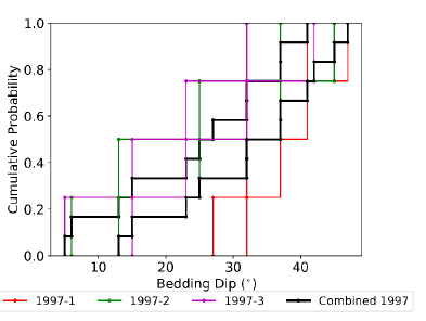
Figure 9 presents a step forward in the evidence combination (updating). Here again, the bedding dip is depicted, but in this case, the updating sequence is shown. First, in black is the already 1997 combined information. Then, in green the information from 1997 aggregated with the data collected in 2011 is shown. Finally, in red is the latter set, now updated with the evidence collected in 2016. With this last robust random set, the updated wedge factor of safety can be computed.
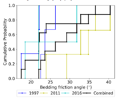
Regarding the friction angle, the amount of information is much smaller, since there is only one piece of information at each period (see Table 5). Because of this, a smaller updated random input set is obtained as can be seen in Fig. 10.
It is important to clarify that as new information is included, the number of input random sets increases. Hence, the number of computations required to define the probability of failure also increases. As an example, for the first piece of information collected in 1997, there were three input random sets, each one with 3 or 4 focal elements, which brings 384 computations of the factor of safety. This number is reduced to 96 since the sensitivity analysis helped to clarify the variation of the factor of safety with the input random variables. When all the evidence is combined, 50176 computations are required, which are reduced to 12544.
This difference in the number of computations does have a relevant influence when more complex computation techniques are involved (e.g., finite elements or discrete elements) since the linked computational cost will constraint the number of computations of the model.
The probability of failure is computed from the bounded distribution function defined for each assessed scenario, as the number of realizations that threw a factor of safety lower than 1.0
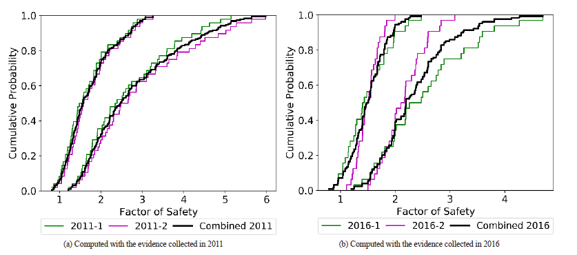
Figure 11 depicts the BDF for the wedge factor of safety computed with the evidence collected in 1997 First, results with the information considered separately are plotted in red, green and magenta for the sources 1, 2 and 3, respectively. These curves reflect the conflict linked to the input parameters, since the factor of safety is highly variable, depending on the considered source of information. The lowest factors of safety are obtained from the first source 1997-1 (red) that has the highest dip and dip direction measurements. On the contrary, the highest factor of safety comes from the piece of evidence 19972 (green), which combines the lowest dip with the lowest bedding dip direction.
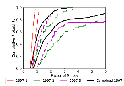
Considering the evidence collected in 1997 separately might lead to a biased conclusion on the actual stability condition of the rock wedge. If the information first collected (1997-1) is involved, a conservative conclusion is drawn, while 1997-2 source could be riskier. This issue justifies the need for combining information, to get a more reliable representation of the actual stability condition.
In Figure 11, the black curves represent the factor of safety obtained when the combined input random sets are considered. These lines balance the biased information provided by independent sources and a result in between the most conservative and the riskiest BDF is obtained. This sort of response is directly linked to the combination rule utilized to aggregate (update) the pieces of evidence, which basically averages the probability assignments of the original random sets.
The averaging effect of the mixing combination rule is much more evident when the input pieces of evidence are more consistent (less conflicting) than those from 1997, which is the case of the information collected in 2011 and 2016. The resulting BDF are plotted in Figs. 12(a) and 12(b), respectively. As can be seen, the combined curves (in black) are located entirely in between the curves gotten from the individual sources. In fact, information collected in 2011 yields the best agreement between BDF computed from individual and aggregated pieces of evidence. These pieces of evidence are the least conflicting (See Tables 5 and 6).
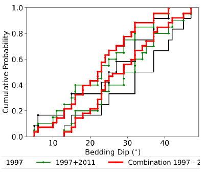
In Figure 13 the factor of safety BDFs resulting from the combination of the information at each period 1997 (red), 2011 (green), and 2016 (magenta) are plotted. There is a noticeable difference, particularly between the results of 1997 and 2011, the earlier is more conservative than the latter.
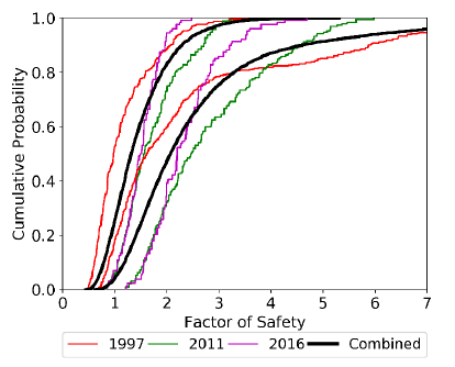
The already aggregated information at every year can be considered as single new pieces of evidence that can be again mixed, to produce more robust input random sets to compute an updated BDF. The result of this task is the BDF plotted in black in Figure 13. That curve subsumes all the information available on input parameters until 2016. Again, the aggregated information balances the results and reflects the nature of the combination rule.
It is also important to remark that when the whole body of information is considered, the probability function, more than discrete, resembles a continuous probability function that might represent a probability box (Ferson et al. 2003). This is because the number of focal elements included for the RST analysis is 28 on bedding geometry and 8 on joint friction angle, so the BDF is the result of 12544 computations of the model.
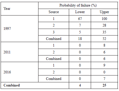
So far, a noticeable difference in the cumulative probability function of the factor of safety has been presented. Now, to make it more objective, the probability of failure when considering different sources of information has been computed and included in Table 7 for FS<1.0. This chart shows different probabilities of failure as different pieces of evidence are considered, e.g., for the information from source 1 in 1997, the probability of failure ranges between 67% and 100%, therefore failure is almost sure. On the other hand, the source 2 of the information collected in 1996 yields a probability of failure of 0, which is not true, since a slope instability was already reported in 2000. When combining all available information, a probability of failure between 4% and 25% is computed.
Conclusions
In this paper, an alternative to compute and update the probability of failure of rock wedges under the random sets theory was presented. The method was applied to a sandstone mine located in Une, Cundinamarca that has been monitored for 20 years and has relevant geotechnical information collected in 1997, 2011 and 2016. The most important findings from this work were:
RST allows obtaining bounded probability curves from the available information, even when this is limited to a few data. Besides, RST allows updating the BDF as new information is available. These two aspects make the RST suitable to be applied in rock mechanics problems where the information is limited, conflicting and new information appears as the project progress.
When the pieces of evidence (or sources of information) were considered separately, noticeable differences in the BDF were obtained, which justified the need for aggregating the information into a representative set of mixed evidence.
The BDF of the factor of safety computed for the combined (updated) evidence balances the results obtained from individual sources and reflects the combination rule utilized to aggregate the different pieces of available evidence. In this case, the applied combination rule was the mixing or averaging.
The sensitivity analysis arises as a powerful tool to reduce the number of variables to be expressed as random sets, which brings a reduction in the total number of realizations to calculate the BDF. This is very important when complex numerical techniques are involved, since its high computational cost constraints the feasible number of model realizations.
Random sets theory, as presented in this paper, is an alternative to systematically include new information in the design process as it is available, which allows to update the model predictions and to assist the decision making at different project stages. Nevertheless, sound engineering judgment is required to define the input random sets.
It is important to highlight that the design of a rock slope is a complex task, in which several mechanisms of failure and triggering factors should be considered. In this context, this research contributes to that complex task by considering the wedge mechanism of failure when limited information from several sources is available. However, further work on random sets applied to rock slope stability is required to extend this approach to more general applications.

