


 English (pdf)
 Article in xml format
 Article references
 Send this article by e-mail
 Cited by SciELO
  Cited by Google
  Similars in
SciELO
Similars in
SciELO  Similars in Google
 Permalink
GPU parallel architecture
GPU multi-core parallel architecture has received more and more attention in the field of high-performance computing in recent years. GPU was originally used for graphics processing acceleration tasks. With the development of general-purpose GPU (General-Purpose Computing on GPU, GPGPU-related) software and hardware platforms, GPUs are gradually applied to parallel acceleration in the field of scientific computing. One of them is NVIDIA. Launched the Compute Unified Device Architecture (CUDA) platform (Appleyard, Appleyard, Wakefield, & Desitter, 2011; NVIDIA, 2009). The algorithm in this paper is based on CUDA implementation.
The GPU achieves higher computing performance by integrating more computing units on the same chip area. Take NVIDIA's Kepler architecture GK110 chip as an example. The most basic computing unit is the CUDA core. A complete GK110 chip contains 2,880 CUDA cores. The K10C GPU with GK110 chip has 5GB GDDR5 (Graphics Double Data Rate, version 5) memory, and its single-precision and double-precision floating-point operation peak speeds are 3.52 and 1.17 TFLOPS respectively (Float Operation Per Second, floating-point operations per second). The peak bandwidth has reached 249.6 GB/s. These metrics far exceed the peak data of the same level of CPU.
GPU parallelism is often memory-constrained, so it must be well-designed to accommodate the GPU's multi-level memory structure to maximize GPU computing performance (NVIDIA, 2012a; NVIDIA, 2012b).
Linear System Solution in Reservoir Numerical Simulation
Control equation
In reservoir numerical simulation, the basic governing equation is the mass mass conservation equation. For any discrete grid system, the mass conservation equation for a certain mesh i and component c can be written as:
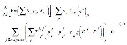
Which represents volume, represents porosity, represents phase saturation, represents phase density, represents component mass fraction, represents source term (well term), represents all meshes connected to i, represents a phase, between a connected mesh Conductivity, which represents pressure, represents the mass density of the phase, represents the gravitational acceleration constant, and represents the mesh depth.
Additional constraints are required to solve the above system. For the most common case, in the constraint equation V represents volume, ø indicates porosity, indicates phase saturation
Equation (4) represents the fugacity balance of the components between phases and .
The above systems are usually solved using the Newton iteration method. At each Newton iteration step, the corresponding Jacobian matrix and the right-end term are obtained, and the linear system is solved, and the Newtonian update is performed until the nonlinear equation converges, and then the simulation of the next time step is performed.
In the above process, the linear system solution takes up the most time. In the reservoir numerical simulation, the Krylov subspace-based iterative solver is generally used to solve such large sparse linear systems. Generalized Minimum Residual (Saad, 2003; Saad & Schultz, 1986) (Generalized Minimum Residual, GMRES) is one of the most commonly used solvers. However, the performance of such solvers depends to a large extent on the pre-processing methods used with them.
CPR two-stage pretreatment method
The equation system of the reservoir problem has mixed characteristics, which are close to the part of the elliptic equation (pressure equation) and the part close to the hyperbolic equation (convection equation). In order to solve this mixed equation problem, Wallis et al. (Wallis, 1983; Wallis, Kendall & Little, 1985) proposed a two-step pretreatment method, Constrained Pressure Residual (CPR). In this method, the first step extracts the pressure matrix from the complete Jacobi matrix, solves the pressure matrix to eliminate the low frequency error existing in the pressure variable, and the second step preprocesses the complete matrix to eliminate the high frequency error (or local error). ). The mathematical characterization and algorithm steps of the CPR method are as follows.
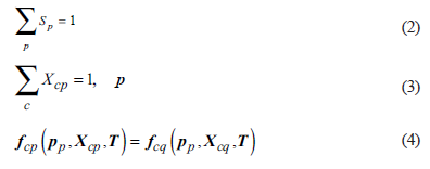
The preprocessing matrix defining the CPR method is M 12
Where M 1 and M 2 are the preprocessing matrix for the first and second steps, respectively. It is the original matrix, which is the unit matrix.
Call CPR method to get x = M -1 1,2 v . It can be broken down into two separate pre-processing processes to calculate:
1) Call the first step of the preprocessing algorithm, calculate x = M -1 1 v;
2) Calculate v 2 = v - Ax 1
3) Call the second step preprocessing method, calculate x 2 = M -1 2 v.
4) Calculate x = X 1 + x 2 .
Reasonable selection of two separate preprocessing methods as CPR components, the CPR method proved to be very efficient in dealing with reservoir simulation problems, on a series of complex models including standard wells, multi-segment wells and unstructured grid models. Can have very good performance (Jiang, 2007; Jiang & Tchelepi, 2009).
The pressure solution process in CPR generally uses the multigrid method (Stüben, 1983), and the global preprocessing stage generally uses the ILU0 method. This paper retains the CPR solution framework and uses the MPNF method as a two-stage preprocessing method.
Nested decomposition
Traditional NF method
The NF method (Stüben, 1983) is a classical linear solution preprocessing algorithm for reservoir numerical simulation problems for structured grids. Its basic idea is to use the nested three-diagonal matrix structure corresponding to the structured mesh to solve the problem quickly. For structured grid systems that are small (within hundreds of thousands of grids), the NF method has high efficiency.
MPNF Method
NF is a completely serial algorithm, both in the decomposition phase and in the solution phase. In order to make it parallel on the GPU, the algorithm needs to have a large number of parallelizable units. MPNF is such a variant.
MPNF achieves good fine-grained parallelism through dyeing and rearrangement. For example, a set of meshes extending in the z direction (other directions are also possible) is called a kernel; then coloring is performed at the core level (that is, the xy plane), and the dyeing operation refers to Each unit is assigned a color, so that adjacent units always belong to different colors; finally, the grid system is rearranged by number, first in color order, and the same color is sorted by core (the order between cores can be arbitrary) ), the core internals are sorted from small to large in the z direction.
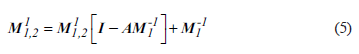
Thus, the inner mesh of the core is a one-dimensional connection, and the numbers are adjacent, resulting in a three-diagonal structure.
Where nC represents the number of grids in each core, representing the serial number of the core. It can be a single element or a dense matrix block, depending on the current matrix type (pressure matrix or main matrix) and the number of implicit variables in each grid block.
The cores in the same color are not connected to each other, forming a block diagonal structure.
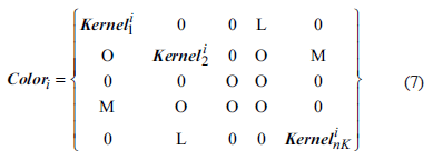
Where nk Represents the number of cores in a color (the number of cores in different colors is generally different), representing the serial number of the color.
Think of a grid within a color as a whole, as long as the dyeing algorithm ensures that the different colors are also one-dimensional connections, then the colors also form a block-like three-diagonal structure.
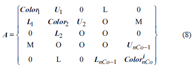
Where nCo representative dye number, L, U Represents the non-diagonal elements produced by the connection between colors.
Compared with NF mehtod, MPNF through dyeing and rearrangement, a matrix of two-level three-diagonal nested structure is formed, and a similar factorization can be performed corresponding to the pre-processing matrix. Since at the color level, the cores inside the same color are always not adjacent, the parallelism is obtained between the cores. In the decomposition and solution phase of the preprocessing, each core can be executed in parallel when it involves operations within each color.
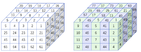
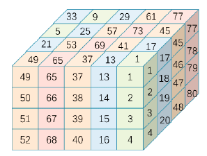
The simplest method of dyeing is the checkerboard dyeing of two colors, alternating the two colors to complete the staining on the plane. As shown in Figure 1. In the figure, each core contains 4 grids, which are arranged in the longitudinal direction. After dyeing, the two colors each contain 10 cores, and the cores in the same color are not connected to each other.
Fewer staining results in higher parallelism, but at the same time the approximation of the preprocessing matrix is degraded, and convergence requires more iterations. Appropriate increase in the number of stains may contribute to the parallel effect as a whole.
A four-color oscillatory format staining method is shown in Figure 2. The dyeing starts from one corner and is sequentially dyed according to the strip parallel to the diagonal, and the color is circulated in the order of 1→2→3→4→3→2→1. Obviously, this dyeing method can still ensure that the cores in the same color are not connected, and the color is a one-dimensional connection. Figure 3 is the corresponding matrix structure.
Efficient implementation and expansion of MPNF methods
Appleyard (2011) describes the principle of the MPNF method, but there is no specific implementation details; Zhou (2012) used the MPNF pre-processed GMRES for the CPR first-stage solution, and introduced the CUDA-based GPU algorithm implementation in detail, and this method Applied to multi-GPU parallelism.
This paper implements a complete GPU parallel linear algorithm based on CUDA. The algorithm uses CPR as the preprocessor and GMRES as the accelerator solution framework. The preprocessor selection of CPR two stages is MPNF method.
Consolidated access
The global memory is the memory outside the GPU chip. It has the largest storage space and the largest access latency. When the algorithm works, it will store all the data that needs to be read and written from the host (host) memory. Copy to the device (device, also known as GPU), stored in the global memory for thread access.
Access to global memory needs to satisfy coalesced access: if an instruction needs to access specific data in global memory, and the access locations of all threads (within the same thread bundle) are consecutive in memory, then the merge access is satisfied. . If the merge access condition is satisfied, only one read operation is required, and all threads in the warp can obtain their respective data; otherwise, each thread must perform a separate read operation to obtain the respective data, which greatly reduces the effective bandwidth.
For the MPNF algorithm, the initial matrix data of the host does not meet the merge access requirements, and needs to be rearranged before being passed to the device for parallel algorithms. The data that the MPNF algorithm needs to use includes: matrix data, unknown vectors, and right-end vectors.
The structure is similar and is illustrated by an example. After the mesh is dyed, the initial structure of the diagonal elements is first sorted by color number (that is, the elements whose subordinate color numbers are small are always in front of the elements with large numbers), the same color is internally sorted according to the core number, and the same core is internally meshed according to the grid. The number is sorted. Finally, if the middle element is a matrix block (for b-MPNF), the matrix blocks are arranged in column priority order.
Since the parallelism of the MPNF algorithm exists between the cores in the same color, the thread responsible for processing different cores should access the contiguous memory under the same operation to satisfy the merge access, so it should be rearranged in the following order: firstly, the order is the same according to the color number. Inside the same color, first arranged in layer order (assuming the core is in the z direction); if the middle element is a matrix block in the same layer, it is arranged in the order of the columns in the matrix block; the positions in the same matrix block are in the order of the core number arrangement.
If the above arrangement order in the same color is denoted as IN_ KERORDER, INBLKORDER, KERORDER, the arrangement before and after rearrangement is changed from "KER ORDER" "IN_KER_ ORDER" "INBLKORDER" to "INKERORDER" "INBLKORDER" "KERORDER".
In short, parallelism exists between cores, and only needs to be sorted by core number in the end, and the other order is unchanged to ensure merge access.
In addition to using the same arrangement, the incoming right-end vectors should be rearranged in the same way, as is the calculated solution vectors. The intermediate variables calculated in this way also have the same order.
Block-based b-EllPack format
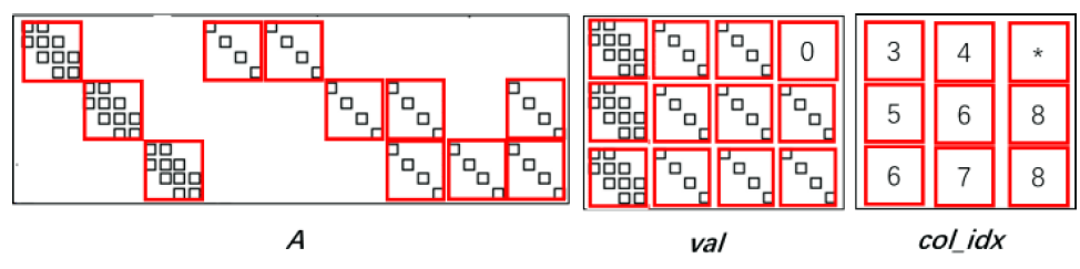
The EllPack format is a sparse matrix storage format, and its storage mode is similar to the CSR format. The difference is that after the matrix is compressed by row, the EllPack format fills 0 elements in rows with fewer nonzero elements so that all rows are compressed to the same length. See Figure 4 for an example of its storage format. Where val is a dense matrix, the number of rows is the same as the number of rows of the original matrix, and the number of columns is the same as the maximum number of non-zero elements in each row of the original matrix, and the position where there is a gap after compression by the row is filled with 0 elements. Val is stored in column priority order. The col_idx storage format is the same as val, recording the original column index of each corresponding position element.
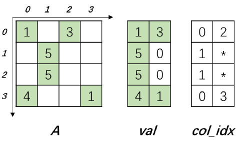
Figure 4 EllPack storage format example. 0 represents the filled 0 element, * represents the subscript corresponding to the filled 0 element, can be any value, will not be accessed when used
When using CUDA for SpMV operations, the operation of each row in the EllPack format is handled by one thread, and the padded 0 element ensures that access to the matrix elements is a merged access. This mode allows it to perform better than the CSR format when the number of non-zero elements in each row is not much different.
In the reservoir numerical simulation problem, the maximum number of non-zero elements per row of the matrix depends on the number of connections of the grid (a grid is connected to at most 6 grids), which is relatively fixed, and after the grid number is determined, the maximum The number of non-zero elements can be calculated, and it is suitable to use EllPack format storage. Combined with the characteristics of the matrix, this format can be further improved.
One of the characteristics of such a matrix is that the first layer of the block structure is constructed in a core organization. In the matrix shown in Fig. 3, the upper non-diagonal element representing the connection between color 1 and color 2 is taken as an example (see Fig. 5), and the red box marked portion represents the connection relationship between the cores of the two colors, and constitutes a connection relationship. A layered structure, in which each small matrix block is a diagonal matrix, which is hereinafter referred to as a core block. Another feature is that each diagonal element in the core block (ie, the black patch in the figure) is also a block structure. With these two layers of block structure, a more compact b-EllPack format can be constructed for SpMV operations.
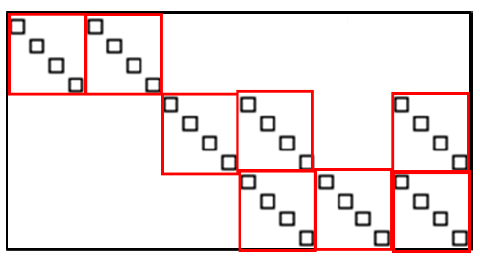
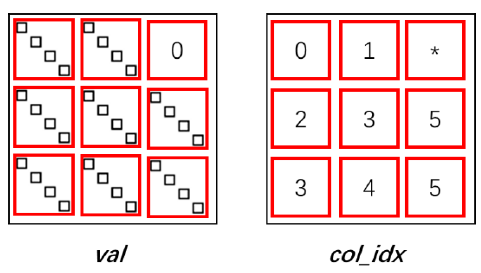
Figure 6 is a schematic diagram of the storage of Figure 5 as a b-EllPack. In this format, only the column subscript of the block block of the core block is stored in col_idx, and the column subscript of each non-zero element is not required to be recorded, and the required storage space and the access frequency thereof are greatly reduced, thereby improving the correlation. The efficiency of the operation. When performing SpMV operation, each thread processes a block operation of a core block. The storage order of specific elements in the val array should be: firstly stored in the order of the block block of the core block; sorted by layer in the block column of the same core block (Assume that the core is distributed along the z direction); the same layer is arranged in the order of the columns of the small matrix blocks; finally, the core blocks are sorted by the block rows.
The matrix representing the connection between colors can be stored in the b-ELLPack format. The SpMV operation needs to be performed when solving the block-shaped three-diagonal matrix composed of colors, and the obtained result vector is used for the right-end term of the inner three-diagonal solution of the next color. Therefore, in addition to the higher efficiency, this format can also make the order of the result vectors obtained by the matrix after the SpMV operation coincide with the order of the right end items required for the inner tridiagonal solution of the color (ie, the order).
For p-GMRES and b-GMRES, the SpMV operation of the pressure matrix and the main matrix is required in the algorithm. A simple modification to the above format is applicable. This variant is hereinafter referred to as the b-Diag-EllPack format.
Take the main matrix as an example. The main matrix differs from that of Figure 5 in that the block diagonal elements are internally trigonal rather than diagonal. The diagonal block always exists, so only the diagonal block needs to be stored in the top position of each block row, and colidx does not need to store the column index of the diagonal block, and the correlation operation is performed. The block column can be specially treated. The order of the special block columns can be various, and it is only necessary to ensure that the order of the last two steps is arranged in the order of INBLKORDER KERORDER.
FIG. 7 is a behavior example corresponding to the first color in FIG. 3, showing the corresponding b-Diag-EllPack storage format.
Correspondingly, the SpMV results of the main matrix are also stored in the same order. When performing other vector parallel operations, they must first be converted back to the normal order.
MPNF method for 2.5d unstructured grid
The simulation of fractured reservoirs uses the Discrete Fracture Model (DFM). The DFM mesh model can be a completely unstructured tetrahedral model or a semi-structured layered model (ie 2.5d). A layered model is a grid system that is still divided into layers in the longitudinal direction and is formed by triangulation (or other splitting format) on the plane. Compared with the tetrahedral model, the layered model has limitations in applicability (requires cracks to be high-angle seams), but it has significant advantages in terms of sectioning difficulty, grid quality, formation information, and speed of solution. An important unstructured grid model.
Kuznetsova et al. (2007) introduced a method of applying the NF method to a layered model: dyeing on a plane to construct a two-layer one-dimensional joint structure (the grid in the same color is a one-dimensional connection, and the color is one between Dimensional links, plus one-dimensional connections in the vertical direction, finally construct a three-dimensional one-dimensional structure in the unstructured grid.
Similarly, the MPNF method itself does not require the distribution of the mesh on the plane: as long as one direction can be selected as the direction of the core extension (requires the same number of core meshes, and is a one-dimensional connection), and in the direction of the core extension A dyeing method can be given on a vertical plane to ensure a one-dimensional connection between colors, and the MPNF method can be applied.
Appleyard (2016) presented a method for staining unstructured meshes on a plane. First select the color number and the stimuli format of the dye sequence; select the starting grid, assign it the starting color; find the current unstained, but at least one of the grids connected to the dyed grid to form a candidate list; statistical candidate list The number of different colors connected to the grid is arranged in descending order of different color numbers; the next color in the color sequence is taken, and the grids satisfying the requirements (the same color cannot be connected) are sequentially given in the order of the candidate list until the traversal is completed. Finally, look for a new candidate list and repeat the above process until all the grids have been dyed.
This is a general dyeing method that works equally well for structured grids. When applied to a structured grid, the number of colors is at least 2; however, when applied to an unstructured grid, the number of colors required is generally large (eg, 6).
Figure 8 is a schematic diagram showing the results of staining on a plane using a dyeing method for the above dyeing method. The unstructured mesh is generated by Triangle (Shewchuk, 2002) (using the -q command to control the triangle element as close to the regular triangle as possible). It can be seen that the dye spreads outward from the layer at the initial grid, and the shock stimuli sequence is still well maintained.
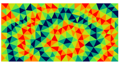
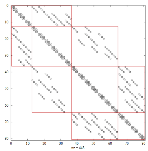
Figure 9 is a layered model (divided into 41 triangular grids on the plane, divided into 3 layers in the longitudinal direction) and rearranged by 6 colors according to the above method, corresponding to the matrix structure diagram. The part marked by the red frame is a three-diagonal structure composed of connections between colors. It can be seen that for non-structural meshes, this method of dyeing does not completely guarantee a one-dimensional connection between colors, so there will be a small amount of elements that fall into the tri-diagonal off-band.
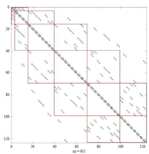
When using MPNF preprocessing, these off-band elements can be ignored. Although there is some loss in accuracy, a strict three-diagonal structure is guaranteed, so that the algorithm can be performed normally. But whether it is the GMRES algorithm in the pressure solution process or the GMRES algorithm used in conjunction with CPR, the SpMV part still uses the exact matrix.
Study Case Test
Algorithm convergence performance and time-consuming analysis
This section selects the first 10 layers of the SPE10 (Van der Vorst, 1992) example, and performs performance test and time analysis on the CPR two-stage MPNF algorithm. The grid size is 60x220x10, a total of 132,000 grids, and the fluid is oil-water two-phase. The MPNF method in the pressure phase is combined with GMRES, that is, the one pressure matrix solution may need to call multiple MPNF solving processes, and the convergence error is set to 0.1; the second phase MPNF is used alone, that is, the second phase MPNF solving process is performed only once per CPR call. .
The first is the test of convergence speed. ILU0 and AMG were selected for comparison with p-MPNF, and BILU0 was selected for comparison with b-MPNF. The MPNF method also selects the number of stains as 3, 4, and 5 for comparison. If the MPNF method is not used in both stages of CPR, the grid number is in natural order. If MPNF is used in any stage, the grid number is the order after dyeing. When ILU0 is used in the pressure solution phase, it is also used in combination with GMRES. The pressure solution convergence error is 0.1, and AMG is used alone. The second phase of BILU0 is also used separately. The test platform hardware is configured for one Xeon X5670 CPU and one K20C GPU.
Table 1 shows the test results. First, the number of Newton iterations is almost the same in all the examples. This is because the selection of the specific components of the linear solution does not affect the Newton convergence speed under the same linear solution strategy and convergence error. The number of linear iterations is the number of iterations of the outer GMRES. CPR preprocessing is called once per iteration. The size reflects the validity of the CPR combination. The CPR combination of the example 1 achieves the best effect, which is consistent with the usual understanding. AMG is best suited as the choice for the stress solution phase in CPR.
Table 1 Comparison of iteration speeds of different CPR combinations (3c, 4c, 5c represent the number of dyes, respectively, 3, 4, 5)
| Study number | CPR combination | Newton iterations | Linear iterations | Pressure solution iteration number | Average number of iterations per iteration |
|---|---|---|---|---|---|
| 1 | AMG+BILU0 | 147 | 667 | 667 | 1.0 |
| 2 | ILU0+BILU0 | 145 | 786 | 25073 | 31.9 |
| 3 | p-MPNF+BILU0(4c) | 147 | 871 | 25770 | 29.6 |
| 4 | p-MPNF+b-MPNF(4c) | 147 | 869 | 25635 | 29.5 |
| 5 | p-MPNF+b-MPNF(3c) | 147 | 941 | 28412 | 30.2 |
| 6 | p-MPNF+b-MPNF(5c) | 147 | 840 | 24501 | 29.2 |
In the comparison between the case 2 and the case 3, the average number of iterations required for each pressure solution is used as a standard, and the ILU0 is used for the pressure solution to be slightly weaker than the MPNF. Considering that the calculation example 3 is based on the dyeing rearrangement, the rearrangement will make the quality of the matrix worse in the sense of solution, and thus the number of linear iterations is more than that of the second example.
Comparing Example 3 with Example 4, the number of linear iterations is very close, reflecting that MPNF as a second-stage preprocessing is similar to BILU0. A comparison of the examples 3, 4, and 5 shows that the increase in the number of stains is beneficial to the matrix solution, whether it is a pressure matrix or an outer iteration. But the difference between the three in this test case is not obvious enough.
First, the MPNF decomposition phase time consumption is negligible compared to the solution phase. This is because for p-MPNF and b-MPNF, the decomposition phase is only executed once for each Newton iteration; and the solution phase for b-MPNF is every time. The CPR call is executed once. For p-MPNF, it is executed once per pressure iteration in each CPR call; the number of times of pressure solution iteration is very large, and the number of executions in the decomposition phase and the solution phase are very different (for p-MPNF and b- MPNF is 1:174 and 1:6) respectively.
BLAS operation has good parallelism, but the computational density is very low (the ratio of the number of memory reads to the number of calculations), which is limited by the GPU bandwidth cannot achieve high performance; the reduction operation decreases rapidly with the parallelism of the algorithm. Also can't have a good performance. The number of these two operations is affected by the number of GMRES iterations. As the number of iterations increases, the number of BLAS and reduction operations performed per iteration increases linearly. Therefore, the two occupy a large proportion in the algorithm time composition.
In order to reduce the general BLAS and reduction operations for parallel performance, the BiCGStab (stabilized double conjugate gradient method) solver can be used instead of GMRES, which is used in conjunction with the pressure matrix solution. BiCGStab is also a subspace iterative method for general matrices. Experience has shown that GMRES is more stable because it guarantees that the norm of the residual is monotonically decreasing after each iteration. However, BiCGStab is different from GMRES in that the number of BLAS and reduction operations does not change with the number of iterations in each iteration. For the problem that the average number of iterations is close to 30, the ratio of these two operations is greatly reduced.
On the other hand, the stress solving phase in CPR does not require high accuracy. Convergence criteria for relaxation stress solving can be considered to reduce the number of iterations of excessive pressure system solutions.
The pressure solution was changed to BiCGStab and the pressure convergence criterion was relaxed to 0.5 and tested again. The comparison results are shown in Table 2. The number of Newton iterations is constant, the number of linear solutions is increased by 40%, but the average number of iterations of the solution is reduced to 11 times, and the total time consumption is reduced by more than 40%. The increase of the number of linear solutions is caused by the lower precision pressure solution, which increases the time consumption of the outer GMRES and b-MPNF, but also reduces the average pressure solution iteration number, and finally reduces the total pressure solution iterations. . In addition, it should be noted that the total time consumption of MPNF has not decreased, but has increased. On the one hand, BiCGStab will call p-MPNF solution twice in one iteration, so that the actual number of p-MPNF calls in two tests is close; The number of b-MPNF calls increases as the number of linear iterations increases, and the time spent on a single call is also higher than that of p-MPNF.
Table 2 Comparison of iterative speeds between different pressure solver selections and convergence errors
| Study setting | Newton iterations | Linear iterations | Pressure solution iteration number | Average number of iterations per iteration | Total time consumption / s | MPNF total time consumption / s |
| p-GMRES ConvP<0.1 | 147 | 869 | 25635 | 29.5 | 48.7 | 11.2 |
| BiCGStab ConvP<0.5 | 147 | 1233 | 13551 | 11.0 | 27.5 | 12.4 |
Thanks to the use of BiCGStab, the proportion of time for reduction and BLAS operations decreased from 59% to 21%. Parallel performance The general proportion of calculated components is reduced, which is the reason for the significant reduction in total time consumption. Under the new setting, the MPNF solution stage time consumption is 44.7% (mainly p-MPNF solution stage, more than 90%), which occupies the main part. At the same time, the proportion of the remaining serial part in the linear solution algorithm is also more significant (close to 20 %). Although this ratio is very high (resulting in an acceleration ratio of up to 5), the main time composition of the serial part is derived from the pressure matrix decomposition process. For more complex problems, a pressure matrix decomposition will correspond to more linear iterations, corresponding strings. The proportion of the line portion will also decrease.
SPE10 study test
This section uses the complete SPE10 model for parallel algorithm testing. The complete SPE10 model consists of60 x 220 x 85 with a total of1.1 million grids. The model hole permeation field height is heterogeneous and is a standard example designed to evaluate the performance of linear solvers. The fluid uses two phases of oil and water. The model consists of four production wells located at the four corners of the model and one injection well located in the center of the model. All wells are shot through all formations. The test platform is the same as before.
This paper implements a serial version of the two-stage MPNF algorithm as a reference to measure the acceleration of parallel implementation. At the same time, the GMRES method preprocessed by CPR (AMG+BILU0) under the serial algorithm is also added to compare the advantages of the parallel algorithm compared with the current mainstream serial algorithm. The comparison is classified according to the total time taken by the linear solution, the time-consuming of the pressure matrix, the second-stage pre-processing and the outer GMRES time-consuming.
The parallel version of MPNF achieved an acceleration ratio of 19.8 over the entire linear solution phase, and an acceleration ratio of 23.9 and 27.0 was obtained in the pressure solution phase and the second phase pretreatment and the outer GMRES, respectively. Since the total speedup includes additional overhead and other parts that cannot be paralleled, it is lower than the other two parts; the second stage preprocessing and outer GMRES are similar in composition to the stress solution stage (average GMRES iterations are 12 times), but thanks to the use of the block matrix, the access limit is smaller, so the acceleration ratio is higher than the pressure solution phase.
The serial version of MPNF is significantly slower than the serial version of the mainstream solution combination. Among them, the velocity matrix solution speed is very different, which verifies that AMG is much better than MPNF in the serial hardware. The pressure matrix solution occupies most of the time (more than 70%) of the linear solution, so although the time consumption of the second stage preprocessing is not much different (about 2 times, the number of CPR calls caused by inaccurate pressure solution increases) Cause), but the total linear solution time is still much higher.
By comparing the latter two, it can be seen that the shortcomings of the MPNF preprocessing method itself can be compensated for on parallel hardware due to better parallelism. The parallel version of p-MPNF is more than twice as fast as AMG, and the serial version of b-MPNF is more than 10 times faster than BILU0. The total linear solution speed is nearly three times faster. This proves the practicability of this parallel solution algorithm, and it can also bring about a real speed increase compared with the optimal strategy of the serial version.
Unstructured equivalent SPE10 study test
This section performs a crack-free layered model MPNF method test. The unstructured mesh (see Figure 10) model is generated based on the SPE10 example, keeping the number of layers unchanged, and the horizontal direction is re-divided into 12,680 meshes, and the attribute field is mapped according to the closest distance of the center point of the mesh. The unstructured model has 1,077,800 grids.
In parallel MPNF vs. serial MPNF acceleration ratio, the structural model has decreased. This is because this study uses 6-color shading, and the number of parallel tasks drops, failing to take full advantage of hardware performance. The average number of iterations for the pressure solution is 20, which is more than the structured model, reflecting the consequences of ignoring elements outside the strip. But the parallel version of MPNF still has an advantage over the AMG+BILU0 combination.
2.5d non-structural example test with cracks
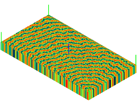
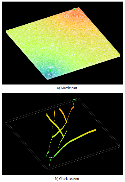
Next is a layered model test with cracks. The model is divided into 10 layers vertically, with a total of 26,418 grids in the horizontal direction, including 417 crack grids. The fracture permeability was 1000 md and the matrix permeability was 1.0 md on average. There is a production well in the two corners of the injection well. The fluid uses two phases of oil and water. The model is shown in Figure 11.
The model uses 6 color stains. The convergence speed information of the MPNF method is shown in Table 3. Although the elements outside the tridiagonal strip are rounded off, the overall convergence performance of the cracked example is still relatively stable. The number of linear iterations is not much higher; the average pressure matrix solution iterations is slightly higher than the regular grid, but it is also within the acceptance range.
Table 3 Comparison of iterative speeds of layered models with cracks
| Newton | Linear | Average number | |
|---|---|---|---|
| Solution strategy | |||
| iterations | iterations | of iterations per | |
| iteration | |||
| AMG+BILU0 | 573 | 9166 | 1 |
| p-MPNF+b-MPNF | 571 | 9953 | 14.8 |
The speedup results are similar to the previous few examples. It is worth noting that the advantage of MPNF compared to AMG+BILU0 combination is more obvious in this example, mainly because the total number of linear iterations is not much different between the two examples.
Conclusion
The linear solution part is the most time-consuming part of reservoir numerical simulation. This paper mainly discusses how to use the GPU as a multi-core parallel architecture to parallelize the linear solution algorithm. Parallel algorithm In the CPR two-step preprocessing solution framework, the MPNF method developed by the classical NF method is selected as the two-step preprocessor selection. The algorithm proposes a data rearrangement method for the two-stage MPNF preprocessing algorithm to ensure the merge access; the block-based b-ELLPACk structure is used to accelerate the SpMV operation in the global GMRES algorithm; BiCGStab is used as the pressure stage solver. The weaker pressure is used to solve the convergence criterion to reduce the proportion of the less conservative reduction operation in the algorithm. Through these optimization methods, the parallel solution algorithm achieves a good parallel effect. Compared with the serial MPNF method, the complete SPE10 algorithm obtains a speed ratio of more than ten times. Compared with the mainstream linear algorithm, it also obtains 2-3. The speedup ratio is doubled.
In addition, this paper uses the general dyeing algorithm to extend the MPNF method applicable to CPR two-stage preprocessing to 2.5 unstructured grid model, which expands the practicability of the MPNF method. In the 2.5d unstructured grid, the dyeing process requires more dyeing numbers, and there are a small number of elements located outside the three diagonal strips. These elements are ignored in MPNF preprocessing, and the parallel effect may be inferior to the structured net. grid. The algorithm was tested on a custom example containing discrete cracks and an example derived from SPE10 mapping (both 2.5d unstructured grid studies). The results were shown on a 2.5d unstructured grid. The MPNF algorithm still has obvious advantages over the serial algorithm.

