


 English (pdf)
 Article in xml format
 Article references
 Send this article by e-mail
 Cited by SciELO
  Cited by Google
  Similars in
SciELO
Similars in
SciELO  Similars in Google
 Permalink
Introduction
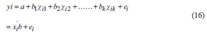
Fitting of data points by parametric curves and surfaces is considered in many scientific fields such as mathematics, statistics, earth and computer sciences. Several standard statistical software has been used by the practitioners to fit the data sets and to estimate the suitable relationships between some response or dependent variable and hypothesized predictor or independent variables (Öztürk, 2014). The researchers want to develop a physical model from an obtained relationship and therefore, they need to determine the value of the response variable based on the estimated relationships. In many situations, however, it is not possible that these types of relationships are valid just by supposing a mathematical model of the relationship. In addition, these variable selection of regression norms cannot be directly applied to contaminated data sets with an ordinary estimation technique. Thus, it is necessary to be collected the data from the population of available data of these variables and then, an empirical relationship between the dependent and independent variables may be estimated from the data (Giloni & Padberg, 2002).
In applied statistics, investigation of the validity of curve fitting methods to fit the observed data is a significant problem. Despite the differences of existing curve fitting techniques, the principal of the most techniques is based on the classical optimization theory and methods. However, the researchers encounter practical curve fitting problems in many quantitative oriented disciplines, and the solution needs to find the most reliable solution to an over determined system of linear equations (Cadzow, 2002). An effective and accurate alternative curve fitting technique has a great importance and serves as a basic module in practice. For this reason, the curve fitting is one of the most common tools in establishing the relationship between a response and an explanatory variable statistic for many social and engineering fields (Durio & Isaia, 2003). The ignoring of a significant component of variability and the equation error is one of the main problems with the usage of the curve fitting models for any data set. Therefore, this problem can lead to either over or under correction for measurement error depending upon the relative sizes of the variances included. The estimation of correlation coefficient for the curve fitting models is a simple tool, and the assessment of the curve fitting can be succeeded by means of the estimation of some criterion such as the calculation of coefficient for the curve fitting model. Many statistical analyzes show that it is not considered as a final model selection criterion. However, this calculation supplies an evidence of the conformity of the selected descriptive variables in estimating the response from the curve fitting model (Renaud & Victoria-Feser, 2010).
In many data processing applications, the linear equation systems under consideration are not consistent and researchers desired to estimate the most approximate solution. Many curve fitting techniques have been used in these types of analyses, for example: Lj Norm or Least Sum of Absolute Deviations Regression (Giloni & Padberg, 2002), L 2 Norm or Least Squares Regression (Cadzow, 2002), Robust Regression (Huber, 1964), Total Least Squares or Orthogonal Regression (Carroll & Ruppert, 1996), Geometric Mean Regression (GMR Leng et al., 2007), Principle Components Regression (PCR, Maronna, 2005), Covariate Adjusted Regression (CAR, Sentiirk & Nguyen, 2006) and Least Trimmed Squares Regression (LTS, Rousseeuw & Leroy, 1987). The main purpose of this study is to estimate the most optimum and reliable curve fitting solutions for linear equations among the earthquake fault parameters of Iranian earthquakes. In this context, a comparison among the first four curve fitting techniques mentioned above was made in order to provide the optimum statistical model between different variables. We did not discuss the other methods such as PCR, GMR, LTS or CAR since they have been preferred in more distinctive applications and they have not generally been used in geophysical analyses. One can also find many details about all these curve fitting techniques in literature (e.g., Branham, 1982; Stefanski, 1991; Hartmann et al., 1997; Spiess & Hamerle, 2000; Shi & Lukas, 2005). Consequently, L t Norm, L 2 Norm, Robust and Orthogonal regressions were tested for Iranian earthquakes in order to provide newer and more suitable empirical relationships among different earthquake fault parameters. By using these different statistical regression techniques, we aimed to make a thorough and consistent appraisal of maximum surface rupture length, maximum surface displacement and associated with the maximum credible earthquakes for different parts in Iran. Also, regional differences in these faulting parameters can be evaluated in terms of geologic, seismic and tectonic variations as the preliminary results of the future studies for the study region.
Mathematical background of the curve fitting methods
Curve fitting problems are classified within the category of mathematical problems, and many different distance functions or metrics have been utilized to carry out linear curve fitting process. There are many mathematical techniques for the solution of these types of problems. However, since our aim is only to evaluate different models and to estimate the optimum relationships, we will not discuss the mathematical background in detailed. For this reason, we will give short and principal explanations for four different curve fitting models in this section, as well as their basic statistical features and quality of fit.
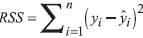
The curve fitting process for a given data set has a great importance in statistical data analysis. These types of data analyses are naturally related to distances in Euclidean geometry and by considering the linear algebra, an analytical result may be possible. Some metrics or distance functions may be useful to perform a linear equation to the data. In order to analyze a linear equation system, it is accepted m observations or measurements on the dependent variable y and some number n ≥1 of independent variables x1.. ..,xn. Each one of them is also known m values. It can be given as (Giloni et al., 2006):
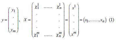
where y Є R is a vector of m measurements and X is an m x n matrix of real frequently termed as the design matrix. In addition, x1.. ..,xn are column vectors with m components and x1,...,xm are row vectors with n components corresponding to the columns and rows of X, respectively. Linear equation system can be formulated statistically as in the following (Durio & Isaia, 2003):

where β T = (β 1 ...... β n) is the vector of parameters of the linear system and ε T =(ε 1 ,......, ε m ) a vector of m random variables corresponding to the error terms in the suggested equation. An upper index T denotes "transposition'' of a vector or matrix. The dependent variable y is a random variable in the hypothesized model. The observations include some "noise' or observation errors and they are taken in the error terms ε. However, we can write it for the linear equation that we want to solve:
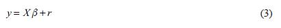
where given several randomly fixed parameter vector β, the components r i of the vector r T =(r 1 ,......,r m ) are the residuals that result, given the measurements y, a fixed design matrix X, and the chosen vector β Є Rn. Consequently, the residuals, r, are in terms of the hypothesized model, realizations of the random error terms e given the particular measurements y and parameter settings β. Given y and X, the main purpose in linear fitting model is to estimate the parameter settings β Є Rp. This means that several suitable measure of the dispersion of the resulting residuals r Є R m must be as small as possible (Giloni & Padberg, 200).
It has completely possible that, e.g., x 1 j = 1, for all j Є {1,......,m} in the design matrix X (Giloni & Padberg, 2002). In this situation, β1 is attributed as the "intercept term" and it is corresponded to the situation in the two parameter case, i.e., when n=2. If x 1 j = 1, for all j Є {1,......,m} and n=1, the problem of estimating a "best" fitting scalar β 1 means that we desire several good measure of "centrality" of the measurements y.
Least Squares Method (L2 Norm)
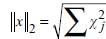
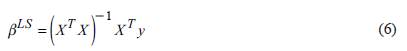
Least squares (LS) method is the most preferred and the best well-known regression technique. This method is the most basic form of the LS optimization problems, and there are many applications in mathematics and statistical data analyses besides other scientific fields. The model estimates β are determined by minimizing the sum of squared residuals under the Euclidean (or L
2
) norm
 , i e. The aim is to estimate the parameters β Є R
p
such that:
, i e. The aim is to estimate the parameters β Є R
p
such that:

must be the minimum. This transformation is uniform and optimality is not affected from it. This minimized equation is positive semi-definite and thus, the first-order conditions achieve the process. For example, in order to minimize S, its gradient ∇S in accordance with β should be computed and adjusted as zero or can be formulated as (e.g., Cadzow, 2002; Giloni & Padberg, 2002):
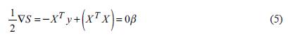
The statement
 should be analyzed for β and is named as normal equations for L
2
norm (Giloni & Padberg, 2002). Supposing that the rank ofXis n, i.e., that r(X)=n, it means that (xTx)-1 exist and the ideal β = β
LS
is stated as:
should be analyzed for β and is named as normal equations for L
2
norm (Giloni & Padberg, 2002). Supposing that the rank ofXis n, i.e., that r(X)=n, it means that (xTx)-1 exist and the ideal β = β
LS
is stated as:
i.e., this regression yields an excellent level. The solution process is focused on the inversion of XTX, but a quantitative analyzer should accomplish the possible singularity of XTX.
The statistical curve fitting techniques have been applied densely for a very long time. Although some significant progress has been made to evaluate the goodness of fit (GOF) besides the other statistical features of the linear curve fitting techniques, some features of the statistical curve fitting techniques require generally poor assumptions (Sen and Srivastava 1990). The estimates β LS in the LS can be accepted as the best estimators when the error terms in the model have a normal distribution. However, the LS estimates depend generally on the presence of the second moment of the error distribution. As a result, this regression model is especially useful for all cases in which involve the analyses of great data sets and handle great samples with the constant numbers of outliers (Cadzow, 2002).
Least Sum of Absolute Deviations Method (L1 Norm)
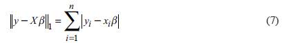
It is well-known that the LS method is very sensitive to unusual measurements in a data. Hence, a large number of robust estimators have been suggested as alternatives, and the least sum of absolute deviations (L 1 ) technique was one of the earliest among them. In this method, coefficients are calculated by minimizing the sum of the absolute values of the residuals. Because L 1 norm can be highly affected by a single measurement, it has been mostly disregarded as a robust alternative to L 2 norm. It has many names in the literature such as LAD (least absolute deviation), LAE (least absolute error), LAR (least absolute residual), LAV (least absolute value), LSAD (least sum of absolute deviations), MAD (minimum absolute deviation), MSAE (minimum sum of absolute errors). L 1 norm has an increasing interest as an alternative to L 2 norm over the past 30 years or so, and it has been a new perspective since 1960s by different researches (e.g., Fama, 1965; Mandelbrot, 1967; Blattberg & Sargent, 1971; Huber, 1987). More descriptive or remarkably illustrative results were provided in many cases by using the L1 norm. The estimates of the parameters β Є R p of the linear curve fitting technique are achieved by minimizing the sum of the absolute residuals (Giloni & Padberg, 2002):
Instead of the L
2
model, L1, model
 is used to minimize dispersion of the residuals. This target function is obviously non differentiable and computation does not assist (Giloni & Padberg, 2002). A significant advantage of L
1
method in comparison with L2 regression is its stability. It is well known that the L1 technique can resist some large errors in the data y for unlimited problem (Shi and Lukas 2005). When a small part of the data being evaluated is not reliable (i.e., contains data outliers), L1 model is suitable. L1 model application may ignore some bad data points if it emphasizes the larger part of data points (Cadzow, 2002).
is used to minimize dispersion of the residuals. This target function is obviously non differentiable and computation does not assist (Giloni & Padberg, 2002). A significant advantage of L
1
method in comparison with L2 regression is its stability. It is well known that the L1 technique can resist some large errors in the data y for unlimited problem (Shi and Lukas 2005). When a small part of the data being evaluated is not reliable (i.e., contains data outliers), L1 model is suitable. L1 model application may ignore some bad data points if it emphasizes the larger part of data points (Cadzow, 2002).
L1 model calculation of β is the solution to the problem for the linear model which has linear constraints:
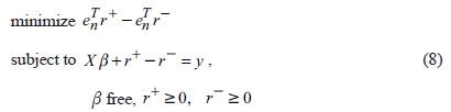
In the equation (8), the residuals r of the general formulation (3) are simply replaced by a difference r+-r of positive variables. The non-differentiability of the exact value target function is dissembled by the target function of (8). However, it accurately captures the target function of L1 norm. Because of the non-differentiability of the criterion function, L1 estimation is more difficult than L 2 estimation. The statistical hypothesis improved for L 1 method is less advanced than it is for L 2 method (Rosenberg and Carlson 1977), whereas
we have the formula
 for the L
2
norm estimates β
LS. It allow us to obtain the sample distribution of [
LS from the error distribution, and the dependence of the L
j
norm estimator on the errors is more complex. The asymptotic theory for L
1
norm is not as well-developed as for L
2
norm. This theory is true to a certain degree. It is also true for high-breakdown model estimators. In addition, L
1
norm estimator is not at all robust to measurements with unusual predictor values; that is, it has a low breakdown point (Giloni et al., 2006). Also, one can see Arthanari & Dodge (1981) for further mathematical background and discussion of the L
1
approach.
for the L
2
norm estimates β
LS. It allow us to obtain the sample distribution of [
LS from the error distribution, and the dependence of the L
j
norm estimator on the errors is more complex. The asymptotic theory for L
1
norm is not as well-developed as for L
2
norm. This theory is true to a certain degree. It is also true for high-breakdown model estimators. In addition, L
1
norm estimator is not at all robust to measurements with unusual predictor values; that is, it has a low breakdown point (Giloni et al., 2006). Also, one can see Arthanari & Dodge (1981) for further mathematical background and discussion of the L
1
approach.
Orthogonal Method (Total Least Squares Method)
Orthogonal regression (OR) is one of the best known methods for errors-in-variables estimation in the simple linear curve fitting technique. This method is also sometimes named as the functional maximum likelihood estimator under the limitation of known error variance ratio. In an ordinary linear curve fitting model, the aim is to minimize the sum of the squared vertical distances between the y data values and the corresponding y values on the fitted line. However, the aim in OR is to minimize orthogonal (perpendicular) distances from the data points to the fitted line.
OR is derived a pure observation error perspective. It is supposed that there are theoretical constants y and X which are linearly related through (Carroll & Ruppert, 1996):

Formulation (9) shows that y and X would be exactly linearly related if they could be measured. In a classical OR technique, instead of measuring (y, X),Carroll & Ruppert (1996) estimated them by corrupted by observation error:
where ε and U are independent mean zero random variables with variances σε 2 and σu 2 respectively. Equations (9) and (10) are combined, the result can be written as:
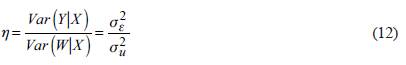
The knowledge of error variance ratio is necessary for OR techniques:
Equation (12) is based on a sample of size
 and the course ofX's are unknown and unobserved. OR estimator is estimated by minimizing:
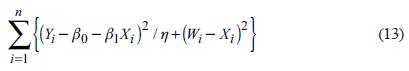
in the unknowns, namely f β
0, β
1, X
1
,......, X
n
. Equation (13) is just the ordinary total Euclidean or perpendicular distance of
 from the line
 . However, equation (13) is a weighted perpendicular distance if
 , and S
wy
are the sample variance of the Y’s, the sample variance of the W’s, and the sample covariance between the Y’s and the W’s, respectively, OR estimate of slope is (Carroll & Ruppert, 1996):
, and S
wy
are the sample variance of the Y’s, the sample variance of the W’s, and the sample covariance between the Y’s and the W’s, respectively, OR estimate of slope is (Carroll & Ruppert, 1996):

This well-known OR estimator is explained in many studies such as Madansky (1959), Kendal & Stuart (1979), Weisberg (1985), Fuller (1987) and Leng et al. (2007). The use of OR must include a careful analysis of equation error and is not only the usual estimation of the ratio of observation error variance. Also, OR fitting technique is an acceptable norm as long as 7 in equation (4) is specified truly. If its assumptions hold, OR is a completely justifiable technique of estimation. Because OR method does not consider equation error, it frequently causes itself to misuse by careless as a technique (Öztürk, 2014).
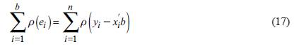
Robust Method
The most important issue in the LS regression is non-robustness to outliers. If the error distribution is not normal, especially if the errors are heavy-tailed, linear LS calculations can produce unexpected results. Especially, if there are extremely incompatible data points, there can be a strong effect on the model parameters by these outliers and we can see it on the results. An easy solution can be obtained by repetitively weeding up these outliers and by calculating again the LS fit for the remaining points. Another method is to operate a different regression model which is not as vulnerable as LS to incompatible data and it is called as Robust Regression (RR). This technique was introduced by Huber (1964), and the best known and common technique for RR is M-estimation. If we take the general curve fitting model in equation (2) into account for the i th of m measurements:
The fitted model is formulated as:
The target function is minimized by the general M-estimator as follow:
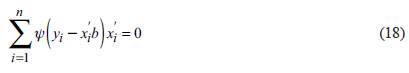
If the derivative of p is accepted as ψ= ρ ', differentiating the target function according to the coefficients, b, and getting the partial derivatives to 0, yield a system of k+1 estimating equations for the coefficients:
If we describe the weight function ω (e) = ψ (e) / e and ω i = ω (e i ), then the estimating equations can be given as follow:
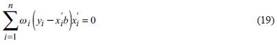
Solving the estimating equations is a weighted LS problem, minimizing
 However, the weights depend upon the residuals, the residuals depend upon the estimated coefficients, and the estimated coefficients depend upon the weights. One can find many details and mathematical backgrounds in Huber (1964).
Nonlinear curve fitting techniques play a significant role in many fields. The classical LS method is generally preferred in many cases for calculating the parameters of a nonlinear model. However, it is well known that these classical techniques are frequently very sensitive to extreme values. Most robust improvements on the estimation of curve fitting model are based on the generalizations of the LS or maximum likelihood methods. RR technique is less influenced by outliers. However, the methods of small sample asymptotes may be very helpful in evaluating the behavior of RR estimates. Several of RR methods are also explained in many studies such as Huber (1981), Field (1997), Sinha et al. (2003) and Abdelkader et al. (2010).
Estimation of correlation coefficient for curve fitting methods
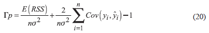
In order to fit mathematical models to measured data, curve fitting applications have been extensively preferred by researchers in many different disciplines. When the error terms identically and independently show a normal distribution, the classic regression method of the LS is efficient. Real data frequently include the extreme values and these data points are covered by a majority of the data while the non-measured random disturbances in a curve fitting method are generally accepted as normally distributed. Many extreme values are controlled by genuinely thick-tailed or asymmetric error distributions, whereas these errors may be the result of observation mistakes or human recording error. Thus, a useful solution for the problem is to minimize the sum of residual error magnitude. If data vector includes a small number of data outliers, the sum of error magnitudes is of particular use in many applications. In these situations, the sum of squared errors criterion is wrongly influenced by these data outliers and therefore often leads to a poor selection of the coefficient vector. In fact, separating the extreme values is not appropriate since they can represent the correct data generating process in these types of situations (Boyer et al., 2003).
The choice of an optimum probability function for a given data set is one of the most significant issues in curve fitting analyses. As seen in literature studies, different methods such as the chi-square test of homogeneity, the test of normality, Kendall and Spearman coefficients, Bayesian Interactive Model, Principal Component Analysis, Mutual Information Coefficient, Hoeffding method etc. can be applied and then, the most appropriate model can be selected. However, there is not any specific rule in the choosing the suitable distribution or parameter calculation methods. The choosing a suitable distribution in many cases is dependent on the GOF assessment. The GOF in a model can be defined as the technique for analyzing how well sample data compatible with an accepted probability distribution (Öztürk, 2014). Some tests for the GOF have been improved and one of the best known and the most frequently used criteria among them is called as correlation coefficient. This term is given as R2 or sometimes r is used, and it has a significant role in curve fitting analyses. As stated in Heo et al. (2008), it is not recommended to be used as a single tool for the GOF, but it can supply an acceptable and quick solution. Although correlation coefficient is only based on the covariance penalty, it is accepted as a substantially simple and effective tool. Alternative models were not used in this study despite many techniques as suggested in literature since these types of applications have been used for more certain fields and they have not been used in geophysical applications.
Considering equation (2), we can assume that
 is the predicted value for yi in the selected model with p<q explanatory variables (based on a LS) and
 is the identical residual sum of squares. Thus, Гp can be given as (Renaud & Victoria-Feser 2010):
As mentioned above, a very simple and practice tool for the GOF is also provided by determination of correlation coefficient for the linear curve fitting models. If we assumed that x is random, we can describe as the parameter which is the squared correlation between y and the best linear combination of the x (Anderson, 1984):

The R 2 is generally given as a quantity and it estimates the percentage of variance of the response variable explained by linear relationship. It is estimated as follow:
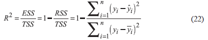
where ESS, TSS and RSS denote the explained, total and residual sum of squares, respectively. If we have an intercept term in the linear model, estimation of R2 is essentially equal to the square of the R2 between y
i
and
 ; , i.e. (e.g., Greene, 1997):

where
 is the average values of the measurements y
i
and
is the average values of the measurements y
i
and
 is the fitted quantiles ,
 . This equation shows that R2 measures the GOF of the linear model by its ability to predict the response variable and its ability measured by the correlation. Moreover, this formulation denotes that the response distribution does not need to be Gaussian to allow for the interpretation of R
2
. It is also a direct estimator of the population parameter of equation (3). The scale and location of R2 do not change and this is statistically independent of the standard deviation and average, y. In fact, R2 supplies a quantitative evaluation of fit and shows the linearity of the probability plot. As an important result, ifR2 is close to 1.0, it is assumed that the measurements can be constructed from the fitted distribution (Heo et al., 2008).
. This equation shows that R2 measures the GOF of the linear model by its ability to predict the response variable and its ability measured by the correlation. Moreover, this formulation denotes that the response distribution does not need to be Gaussian to allow for the interpretation of R
2
. It is also a direct estimator of the population parameter of equation (3). The scale and location of R2 do not change and this is statistically independent of the standard deviation and average, y. In fact, R2 supplies a quantitative evaluation of fit and shows the linearity of the probability plot. As an important result, ifR2 is close to 1.0, it is assumed that the measurements can be constructed from the fitted distribution (Heo et al., 2008).
Data catalog of Iranian earthquakes and a brief definition of the seismotectonics
The first aim of this study is to prepare a uniform data catalog taking the types of surface wave magnitude (Ms) and moment magnitude (Mw) into consideration. Then, the second aim is to estimate the new empirical relationships among the seismicity parameters of different earthquake faulting mechanisms such as Mw and surface rupture length (SRL), Mw and maximum displacement (MD), and SRL and MD. The data set used in the scope of this work is updated form Ghassemi (2016). Table 1 shows the details of parameters for different faulting mechanisms and is modified from Ghassemi (2016). He used 46 Iranian earthquakes whose magnitudes vary from 5.8 to 7.8 and which occurred between the time intervals 1900 and 2014 (Figure 1). As an initial step in Ghassemi (2016), a catalog of Iranian earthquakes related to direct loses was used and the number of initial earthquake catalog was reduced to 41 events. Then, 5 more events were also added to complete the catalog and to extend it to 2014. The outcomes in the present study may differ from specific earthquakes which are used to estimate the relationships between Mw and SRL, Mw and MD, and SRL and MD since this catalog is not complete for SRL and MD. In general, magnitude scale is given as Ms in the original Iranian earthquake database. This data set includes 166 events for Ms and Mw types between 1962 and 2004. In order to prepare a uniform catalog covering Mw scale, new relationships between Mw and Ms were firstly obtained and then, the other empirical relationships among the faulting parameters were formulated by using the most suitable curve fitting technique. One can see Ghassemi (2016) for many details such as the geometry and kinematics of surface ruptures, the secondary ruptures associated with earthquake faulting mechanism, seismic properties of earthquake faulting and the previous relationships among these variables.
Table 1 Data set of fault parameters for Iranian earthquakes between 1900 and 2014 (for details, see Ghassemi, 2016). RLSS: right lateral strike-slip, LLSS: left lateral strike-slip, NF: normal fault, TF: thrust or reverse fault, SRL: surface rupture length, MD: maximum displacement, VDC: vertical displacement component, HDC: horizontal displacement component
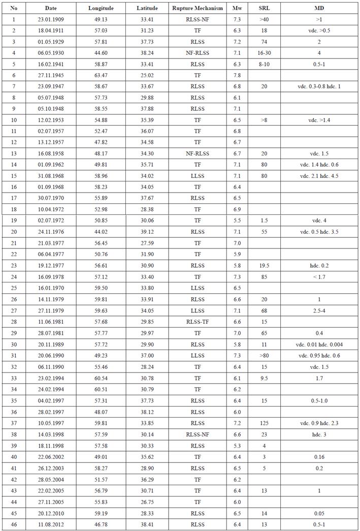
Iran is located within the Alpine-Himalayan orogenic belt in the active collision zone between the Eurasia to the north and Arabia to the south. The Iranian Plateau is consisted of different tectonic systems such as transpressive fold-and-thrust mountain belts with active strike slip and reverse faulting, an active subduction zone and recent volcanic activity; as a result, the plateau shows different crustal blocks of variable thickness and rigidity interspersed by relatively stable aseismic blocks of different sizes (Berberian, 2014). The Iranian Plateau shows active deformation, high elevation and earthquake activity with complex interactions of active strike-slip faults and thrusts, and different destructive earthquakes recorded in historical and instrumental periods. The most significant tectonic structures are mostly accommodated by shortening and strike-slip faulting in the mountain belts and can be given as the Great Caucasus, Zagros, Alborz, Kopeh-Dagh, active Makran subduction zone and also Azerbaijan (northwest Iran) seismotectonic province (Javidfakhr et al., 2011). Along the Iranian Plateau, fault ruptures from earthquakes show a large-scale typical changes and evaluation of them supply many practical understanding for surface rupture hazard in Iran (Ghassemi, 2016). It is well known that Iran was struck with strong and destructive earthquakes in the past and recent years and these earthquakes caused large damages and high loses in human life. Some of these earthquakes are 1909 Silakhor earthquake (Mw7.4), 1945 Makran earthquake (Mw8.0), 1968 Ferdows earthquake (Mw7.4), 1990 Manjil-Rudbar earthquake (Mw7.4), 2013 Ghosht (Mw7.7) earthquake. As a remarkable result, since this study does not include a seismotectonic evaluation or discussion on the earthquake fault rupture hazards in Iran, we did not give many details for the tectonic structures and seismicity of Iran. Thus, a brief and general information is provided in this section. Many readers can reach the knowledge on these subjects from different studies such as Mirzaei et al. (1997), Masson et al. (2005), Djamour et al. (2010), Ghassemi (2016), Öztürk et al. (2017).
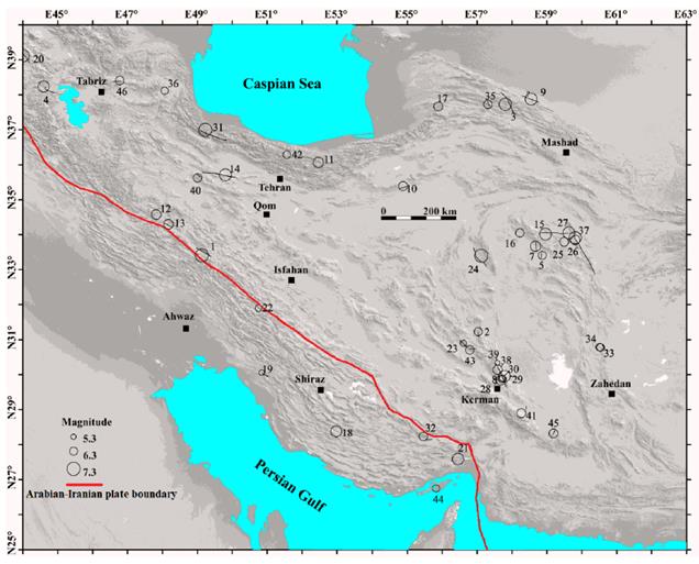
Figure 1 Map showing locations of the earthquake events discussed in this paper. Numbers refer to the event numbers in Table 1. Circles show instrumental epicenters of the events. Where present, surface ruptures are shown in black lines. Instrumental epicenter for the Event No. 6 in Makran region lies outside the map area in Pakistan’s coast. Modified after Ghassemi (2016).
Results and discussions for the applications of alternative curve fitting methods
The main purpose of this study is to provide the new, up-to-date and reliable empirical relationships between Mw and Ms, Mw and SRL, MD and Mw, and MD and SRL considering the parameters of surface ruptures for Iranian earthquakes. In this scope, we used different regressions models such as L 1 , Orthogonal and Robust for different earthquake faulting mechanisms (strike-slip and thrust or reverse faults) in Iran. As stated in Öztürk (2014), measurements of surface ruptures generally accompany many large earthquakes and the logarithms of their length are linearly related to earthquake size. These empirical relationships can supply not only fault sizes for a specific magnitude, but also the maximum magnitude based on these sizes. Such types of results are also very useful for geotechnical, seismic risk and hazard, and seismotectonic studies. Many authors estimated these types of relationships between magnitude and earthquake faulting parameters for different parts of the world (e.g., Acharya, 1979; Wells & Coppersmith, 1994; Ambraseys & Jackson, 1998; Oztiirk, 2014; Ghassemi, 2016).
Ghassemi (2016) preferred the LS method for the analyses and provided several empirical relationships among Mw, MD and SRL based on different earthquake faulting mechanisms in Iran. In addition to the LS method, three different regression applications were used in this study for the same data in Ghassemi (2016). A comparison between the results of Ghassemi (2016) and the results of present study were given in Table 2. Many researchers in various scientific and engineering disciplines have used these types of curve fitting methods in order to estimate the mathematical formulation for observed data points. If we have an unusual error distribution in a data set, linear LS method cannot provide a good estimate (Öztürk, 2014). Therefore, the minimizing the sum of residual error size will be a more preferable and proper definition of the solution. For this purpose, correlation coefficients of the curve fitting models can be preferred as a trustworthy and acceptable tool in the evaluation of the results. As given in Table 2, OR technique provides stronger correlation coefficients than those of the other regression techniques in most estimates expect a few ones. A few poor correlation coefficients, for example R2=0.299 between MD and Mw, and R2=0.411 between MD and SRL, were obtained in the estimations. However, these relationships can be suggested in the evaluation of seismic hazard in Iran. Ghassemi (2016) stated that these types of estimations are related to seismicity analyses and these relationships evidently present the probable range of versatility of faulting parameters. In addition, these relationships may supply an understanding to excessive limits for rupture hazard evaluations, and they may give practical insights in paleo-seismological surveys on active faults of the Iranian Plateau.
Table 2 Empirical equations with LS method of Ghassemi (2016) and all regression fits derived in this study. SS: strike-slip, TF: thrust or reverse fault, All: including SS+TF. Standard errors for all equations are also given.
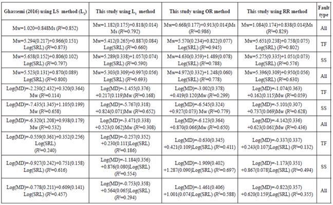
Table 2 shows the comparison of the empirical relationships calculated in this study with the relationships of Ghassemi (2016). Graphical representations of the whole empirical relationships obtained in this study with three regression models and their confidence intervals between Mw and Ms, Mw and SRL, MD and Mw, and MD and SRL were also plotted in Figures 2, 3 and 4. The first numbers in the equations show the error terms and standard deviations of them (in parentheses) and the second numbers show the slopes of the related distributions and their standard deviations (in parentheses), respectively. Considering three curve fitting methods in addition to the LS method by Ghassemi (2016), the suggested linear-linear, log-linear and log-log relationships were given as the more reliable and optimum by OR method with their R2 in the following forms:
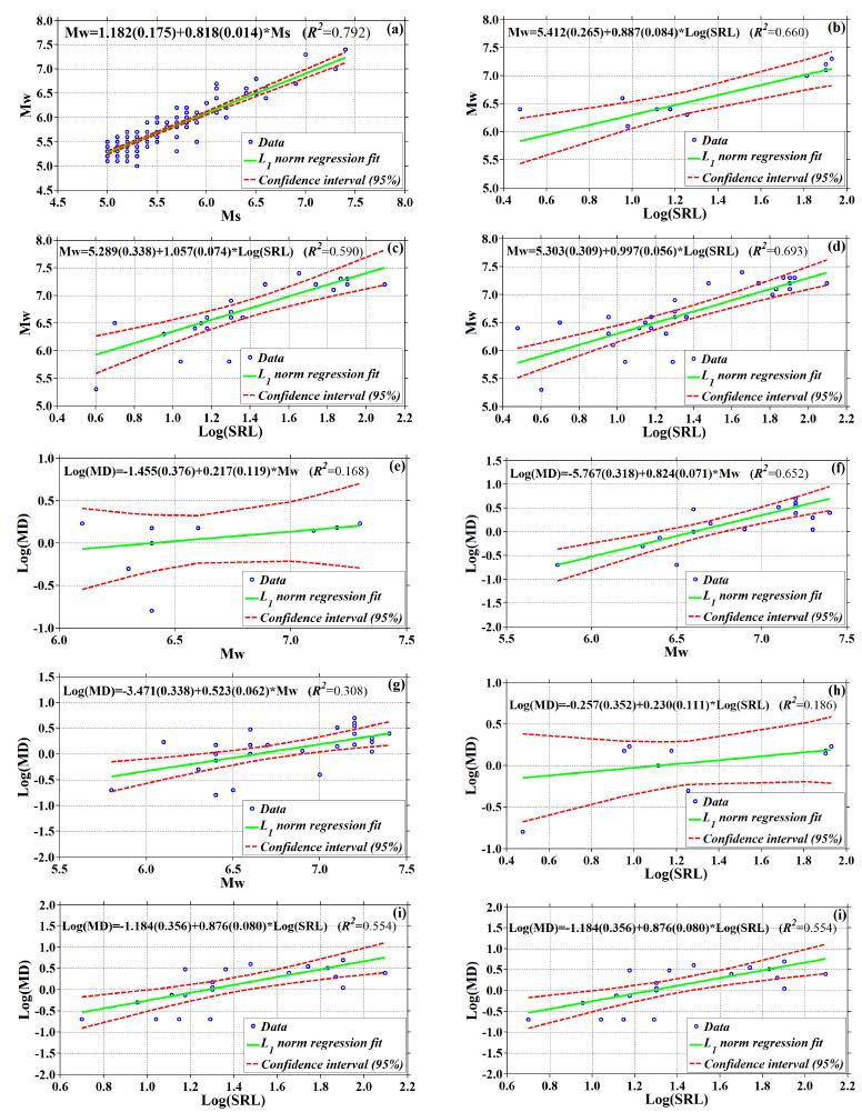
Figure 2 Estimated relationships with Least sum of absolute deviations (L 1 ) method between (a) Mw and Ms for all faulting types, (b) Mw and SRL for thrust and reverse faults, (c) Mw and SRL for strike-slip faults, (d) Mw and SRL for all faulting types, (e) MD and Mw for thrust faults, (f) MD and Mw for strike slip-faults, (g) MD and Mw for all faulting types, (h) MD and SRL for thrust faults, (i) MD and SRL for strike-slip faults, and (j) MD and SRL for all faulting types.
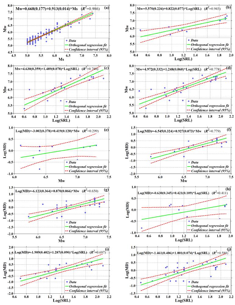
Figure 3 Estimated relationships with Orthogonal regression (OR) method between (a) Mw and Ms for all faulting types, (b) Mw and SRL for thrust and reverse faults, (c) Mw and SRL for strike-slip faults, (d) Mw and SRL for all faulting types, (e) MD and Mw for thrust faults, (f) MD and Mw for strike slip-faults, (g) MD and Mw for all faulting types, (h) MD and SRL for thrust faults, (i) MD and SRL for strike-slip faults, and (j) MD and SRL for all faulting types.
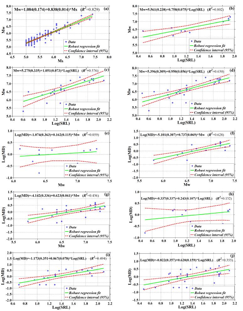
Figure 4 Estimated relationships with Robust regression (RR) method between (a) Mw and Ms for all faulting types, (b) Mw and SRL for thrust and reverse faults, (c) Mw and SRL for strike-slip faults, (d) Mw and SRL for all faulting types, (e) MD and Mw for thrust faults, (f) MD and Mw for strike slip-faults, (g) MD and Mw for all faulting types, (h) MD and SRL for thrust faults, (i) MD and SRL for strike-slip faults, and (j) MD and SRL for all faulting types.
Mw=0.668(±0.177)+0.913(±0.014)*Ms, for all earthquake mechanisms (R 2=0.986)
Mw=5.570(±0.234)+0.822(±0.077)*Log(SRZ,), for thrust and reverse faults (R2=0.945)
Mw=4.630(±0.359)+1.489(±0.078)*Log(SRL), for strike slip faults (R 2=0.788)
Mw=4.972(±0.332)+1.248(±0.060)*Log(SRZ,), for all fault mechanism (R 2=0.778)
Z,og(MD)=-3.002(±0.378)+0.419(±0.120)*Mw, for thrust and reverse faults (R2=0.299)
Log(MD)=-6.545(±0.324)+0.927(±0.073)*Mw, for strike slip faults (R2=0.779)
Log(MD)=-6.123(±0.364)+0.870(±0.066)*Mw, for all fault mechanism (R 2=0.650)
Log(MD)=-0.630(±0.345)+0.421(±0.109)*Log(SRL), for thrust and reverse faults (R2=0.411)
Log(MD)=-1.909(±0.402)+1.287(±0.090)*Log(SRL), for strike slip faults (R 2=0.697)
Log(MD)=-1.461(±0.406)+1.001(±0.074)*Log(SRL), for all fault mechanism (R 2=0.588)
The selection of the confidence interval is quite optional and 90%, 95% or 99% are frequently selected in practice, however, 95% is used in general. As stated in Öztürk (2014), confidence intervals are designed to define the statistical properties of data and are may be used practically in many case. Thus, confidence intervals for all types of regression relationships are selected as 95% in this study. As seen in Table 2 and Figures 2 to 4, correlation coefficients of three regression fits are almost the same for the relationships between Mw and SRL in L2 norm (R2=0.797) and OR method (R2=0.788) for strike slip faults, and between Mw and SRL in L2 norm (R2=0.800) and OR method (R2=0.778) for all faulting types. Regional differences in SRL for a given magnitude can be commented in terms of the local changes in geologic, seismic and tectonic activities. These results suggest that seismic efficiency in a region can be dependent on the rupture length or magnitude. Also, if and when the error terms in the linear regression model follow a normal distribution, then the least squares curve fitting technique is better estimator under the most appropriate criteria. Traditional LS estimation is sufficient when error terms show an independently and identically distribution. However, the LS estimates can give bad fit when error distribution is abnormal. The usage of any curve fitting criterion is preferred when it was doubtful that a small part of the data which is analyzed includes data outliers and thus is not reliable. Curve fitting criterions have the capability of strongly ignoring some bad data points while selecting the majority of data points which put forth the true nature of the data more suitable. The minimizing the sum of residual error magnitude is a reasonable and helpful process for the solution of problem. If the dataset contains a small number of data, the sum of error magnitudes is of particular use and in these situations, these data outliers extremely influence the sum of squared errors criterion. However, the sum of error magnitudes tends to ignore the data outliers on condition that they have relatively few numbers (Öztürk, 2014). Also, Öztürk (2012) suggested for the statistical regression techniques on different dataset that representation of empirical relationships can be made as more appropriate and trustworthy with Least Sum of Absolute Deviations or Robust Regressions for the clustered data while it can be more suitable and reliable with Least Squares or Orthogonal Regressions.
To investigate the maximum surface rupture length (MSRL) and the related maximum credible earthquakes (MCE) in Iran, we studied major earthquake sources in different seismotectonic regions in conjunction with the empirical relationships by OR method of our research. The resulting data were summarized in Table 3. The values are different from those of Ghassemi (2016) in some respects as a result of differences in revised selected earthquake sources as well as difference in the applied regression methods.
Table 3 Maximum surface rupture length (MSRL), maximum surface displacement (MSD), and related maximum credible earthquakes (MCE) suggested for different seismotectonic regions of Iran. See text for further explanation.
* Length quoted for Makran is rupture length at depth
As it is noticed for the analysis of data on surface ruptures of thrust (and reverse) faults using OR method (Figure 3b), the regression line has a small slope with a coefficient of 0.945. This may be partly because of rarity of data on surface ruptures associated with thrust events. As a result, it appears that the relationship may underestimate the earthquake magnitude for major (long) thrust faults, especially when value of SRL is used for blind and/or deep-seated faults. To compensate for such apparent deficiency, we have used the positive side of the standard errors in SRL-magnitude equations for estimation of MCE resulting from active thrust faulting in different seismotectonic regions of Iran. Considering our objective to estimate the MCE for each region, the biggest potential seismic sources are picked for each region. Therefore, it should be kept in mind that in dealing with any seismic hazard approach which does not involve such extreme seismic sources, the MCE would be less than the suggested values in this section (i.e. values in Table 3).
A major potential seismic source in the Kopeh-Dagh region is the Maraveh-Tappeh thrust fault (ca. 260 km long). Considering a rupture which involves half the length (130 km) along the geological fault, a maximum magnitude (MCE) of ca. 7.7 is suggested for the Kopeh-Dagh region. The AshkAbad fault, which forms the northern border of the Kopeh-Dagh geological province within the Turkmenistan territory, is apparently capable of producing earthquakes of magnitudes as large as 8.2 (e.g. the 1895 Krasnovodsk-Uzun Ada earthquake; Ambraseys, 1997).
North of Central Iran, Alborz and Azerbaijan region include major strike-slip and thrust faults which are capable of great earthquakes. These include the Doruneh, Meyamey, Torud, Astaneh, Mosha, Eivanekey, Ipak, Soltanieh and Tabriz faults, among many other. Length of the above-mentioned faults and/or their segments attain lengths up to 170 km, and some of them have produced historical earthquakes as large as magnitude 7.9 (the 856 Kumesh earthquake; Ambraseys & Melville, 1982). Therefore, we consider a magnitude 8.0 as the MCE for the northern Central Iran, Alborz and Azerbaijan region.
Within the Zagros region (except for the High Zagros region) emergent geological faults are rare, and therefore most of attempts for earthquake hazard analyses use folds above blind thrust faults as the source for potential earthquakes. As a result, the surface rupture length used in the related calculations, in fact is not really on the surface but it is related to rupture of a blind fault at some depth (see Berberian, 1995). Following the same approach, we have considered the Kabir-Kuh anticline as the biggest seismic source in folded Zagros region with a length of 166 km, and anticipating rupture of half of the related thrust fault (83 km), an MCE of 7.5 is suggested for Zagros folded region. Therefore, we suggest that for the Zagros folds (and related faults) which are longer than the suggested value in Table 3, the related maximum SRL of 83 km to be used for deterministic evaluation of the magnitude attributed to the fold seismic sources.
The Eastern Iran seismotectonic region is dominated by active strike-slip faulting, and less frequent thrust faults. Surface ruptures are highly manifested in this part of the country as compared to other seismic regions. As a result, relationship between SRL and magnitude in this region shows a greater slope, therefore we have used OR method without including an upper standard error limit to estimate MCE. No historical or instrumental earthquake greater than 7.3 has been reported for the region, therefore we used a maximum length of ca. 100 km for OR of all fault type, suggesting a MCE of magnitude 7.5 for the Eastern Iran region.
Central Iran region has a very low seismicity as compared to other parts of the country, and no historical or instrumental record of earthquakes greater than magnitude 6.2 has been reported for this region. Therefore, a MCE of 6.5 appears to be appropriate for the region.
The greatest earthquakes in the Makran region may occur on the subduction zone at depth. The whole length of the subduction zone is ca. 850 km, which if half of the whole length (425 km) is combined with a width of 180 km and a related 20 m of average displacement, gives a MCE of magnitude 9.1.
We made a comparison for two important relationships suggested for global and Iranian earthquakes, including SRL-Mw (Figure 5) and SRL-MD (Figure 6) relationships. Slope of our regression line for SRL-Mw relationship greatly conforms to those of Nowroozi (1985) and Wells and Coppersmith (1994), however it is less than that of Ghassemi (2016) (Figure 5). A similar comparison between the graphs for SRL-MD indicates that slope calculated in this study is very similar to those of Nowroozi (1985) and Wells & Coppersmith (1994), however the regression has a lower intercept value than those of aforementioned studies. As seen in Figure 6, both slope and intercept values of our study are smaller than that of Ghassemi (2016).
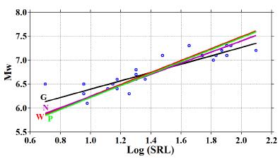
Figure 5 Comparison among different regressions of moment magnitude (Mw) versus surface rupture length (SRL in km) for Iranian earthquakes of all rupture mechanisms (26 events). P: present study, W: Wells and Coppersmith (1994), N: Nowroozi (1985), G: Ghassemi (2016).
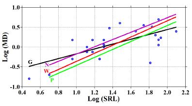
Figure 6 Comparison among different regressions of surface rupture length (SRL in km) versus maximum displacement (MD in m) for Iranian earthquakes of all rupture mechanisms (24 events). P: present study, W: Wells and Coppersmith (1994), N: Nowroozi (1985), G: Ghassemi (2016).
Many studies were made for surface rupture hazard in Iran and some empirical relationships were provided among different earthquake faulting parameters by different researchers such as Berberian (1976), Nowroozi (1985), Wells & Coppersmith, (1994), Berberian (2014), Ghassemi (2016). The only comprehensive analysis of Iranian earthquakes was made by Nowroozi (1985). Also, more detailed quantitative assessments of surface rupture hazard of Iranian earthquakes including historical and instrumental period were provided with Berberian (2014) and Ghassemi (2016). When we compared the empirical relationships estimated in this study with the most up-to-date relationships of Ghassemi (2016), the results in this study present higher R 2 among magnitude and different faulting parameters in OR method. Correlation coefficients of the relationships in Ghassemi (2016) changes between 0.114 and 0.873 with L 1 norm, whereas correlation coefficients with OR technique in present study vary from 0.299 to 0.986. From the observations in this study and in Ghassemi (2016), we can conclude that these estimations for OR method can be thought as good and reliable relationships, and one can use them for the other seismicity analyses or rupture hazard evaluations of the Iranian Plateau. As a remarkable result, we did not make a detailed discussion on the earthquake fault rupture hazards in Iran since this study does not aim to evaluate and discuss this subject. Many details can be found in Ghassemi (2016) for the insights of earthquake surface rupture hazards. For this reason, a short and general comparison of three different curve fitting techniques is provided for the data of Ghassemi (2016). Furthermore, the effectiveness of the different estimation techniques was examined in this study and the relative predictive validity of four regression techniques was compared for different faulting parameters. These detailed analyses show that empirical relationships estimated by OR method in the present study can be thought and used as more appropriate and more trustworthy for Iranian earthquakes and the other mentioned applications. We finally hypothesized that OR estimation technique can provide more stabilized interpretations for the rupture properties, variability of the earthquake fault rupture geometry and kinematics by using these empirical relationships among different faulting parameters.
Conclusions
This study focused on the applications of different regression techniques and a comparison of the empirical relationships of the data set on the surface ruptures of Iranian earthquakes was made. Using a database of Iranian earthquakes, some empirical relationships were estimated among different parameters such as moment magnitude, surface wave magnitude, surface rupture length and maximum displacement for different faulting types. For this purpose, three curve fitting methods are applied as (a) Least Sum of Absolute Deviations, (b) Robust Regression and (c) Orthogonal Regression. In order to decide how we can select the best curve fitting method for a given data set, we calculated separately the correlation coefficients for the thrust or reverse faults, strike slip faults and all faulting types since it is an easy applicable and a practical technique. For the analyses, 46 strong and large earthquakes with magnitudes ≥ 5.8 between 1900 and 2017 were used. In order to estimate the statistical properties of different data sets, 95% confidence intervals were used for each regression relation. Using the above-mentioned techniques, we derived linear relationships among different faulting parameters for Iranian earthquakes. Correlation coefficients varies from 0.299 to 0.986 with Orthogonal regression, from 0.168 to 0.792 with L 1 regression, from 0.059 to 0.829 with Robust regression. These results show that Orthogonal regression fits give more powerful coefficients and can be thought more suitable equations as compared to the other curve fitting techniques.
Resulting equations are proposed as more suitable and reliable in the estimation of the maximum surface rupture length, maximum surface displacement and associated maximum credible earthquakes for different areas of Iran. As a general conclusion, detailed analyses for the data sets of different faulting mechanisms show that more appropriate, more trustworthy more up-to-date representations of empirical relationships can be done with Orthogonal regression. In addition, these types of relationships may supply significant insights in the estimation of the maximum surface rupture length, maximum surface displacement, and associated maximum credible earthquakes for different seismotectonic regions of Iran. We suggested that these relationships may also provide important outputs in the estimation of earthquake magnitudes in paleo-seismological studies.

