DOI: http://dx.doi.org/10.18180/tecciencia.2015.19.8

Comparison and validation of turbulence models in the numerical study of heat exchangers

Comparación y validación de los modelos de turbulencia en el estudio numérico de los intercambiadores de Calor

Juan Gonzalo Ardila Marín¹, Diego Andrés Hincapié Zuluaga², Julio Alberto Casas Monroy.³

¹ Instituto Tecnológico Metropolitano, Medellín, Colombia, Juanardila@itim.edu.co
² Instituto Tecnológico Metropolitano, Medellín, Colombia, diegohincapie@itim. edu.co
³ Instituto Tecnológico Metropolitano, Medellín, Colombia, iuliocasas@itm.edu.co

^* Corresponding Author. E-mail: Juanardila@itim.edu.co

How to cite: Ardila Marin, J.; Hincapie Zuluaga, D.; Casas Monroy, J. Comparison and validation of turbulence models in the numerical study of heat exchangers, TECCIENCIA, Vol. 10 No. 19., 49-60, 2015, DOI: http://dx.doi .org/10.18180/tecciencia.2015.19.8

Received: June 26 2015 Accepted: August 10 2015 Available Online: September 8 2015

Abstract

This study aims to validate numerical models for heat exchangers developed with the commercial package ANSYS®, comparing the results with data published in the literature. The methodology was based on the identification of programs, languages, mathematical models, and numerical models used by other researchers. Geometries were developed with SolidEdge® and DesignModeler®, discretization meshes with Meshing®, and subsequent configuration of standard k-ε and k-ω models with Fluent® and CFX®. For internal flow in concentric smooth straight tube exchangers, we recreated the predicted results with Nusselts varying between 100 and 250 and Reynolds regimes between 12*10³ and 38*10³. The study of internal flow in the curved corrugated tube exhibited considerable approximation to the results predicted by Zachar's numerical correlation with Nusselt numbers in the range of 15-70 for Dean variations between 1*10² and 11*10² in laminar flow. Likewise, we validated the study of external flow in twisted curved tubes. Finally, Nusselt variations between 60 and 275 for Dean variations between 1*10³ and 9*10³ were modeled for completely developed laminar, transitional, and turbulent flow. The study shows the increase of heat flux associated with the change in the geometry of heat exchangers. It also demonstrates how numerical computer models can recreate realistic process conditions and thermo-fluid simulation by appropriately configuring systems.

Keywords: Turbulence, SIMPLE, CFD, wall's law, Nusselt, ANSYS.

Resumen

El presente estudio busca validar modelos numéricos de intercambiadores de calor desarrollados con el paquete comercial ANSYS® comparando sus resultados con los obtenidos en estudios experimentales y numéricos previamente publicados. La metodología se basó en la identificación de los modelos matemáticos, métodos numéricos y programas o lenguajes empleados por varios autores. Se desarrollaron las geometrías con SolidEdge® y DesignModeler®, la discretización en mallas con Meshing® y posteriormente se configuraron en CFX® y Fluent® los modelos k-ε estándar y k-ω. Para flujo interno en intercambiadores concéntricos de tubo recto liso, se lograron recrear los resultados predichos donde el número de Nusselt varía entre 100 y 250 para Reynolds entre 12*10³y 38*10³ El estudio de flujo interno en tubo curvado corrugado con las mismas herramientas logró gran acercamiento a los resultados predichos mediante la correlación numérica de Zachár para Nusselt entre 15 y 70 y variaciones de Dean de 1*10² a 11*10² en flujo laminar. Así mismo, fue validada la independencia de resultados en el estudio de flujo externo en tubo curvado torsionado. Se modelaron variaciones de Nusselt entre 60 y 275 para variaciones de Dean de 1*10³ a 9*10³ para flujo laminar, transicional y turbulento completamente desarrollado. El estudio muestra el incremento en la transferencia de calor asociado al cambio en la geometría en intercambiadores de calor, y muestra cómo con modelos numéricos computarizados se pueden recrear las condiciones realísticas de procesos y sistemas termo-fluidos configurando apropiadamente las simulaciones.

Palabras clave: Turbulencia, SIMPLE, CFD, ley de pared, Nusselt, ANSYS.

1. Introduction

Some studies have carried out experimental analyses on the rate of heat transfer in heat exchangers while many others have been dedicated to numerical analyses of such devices. When designing experimental banks, one can simulate the conditions that would be present in natural or industrial processes. Likewise, when configuring the simulation, models are selected which are the most complex and use the least quantity of simplifications. Such models have given results that come close to those obtained via experiments but require high computing power.

For example, in 2006 Vimal Kumar et al. studied the flow and thermal development in the tube-in-tube helical heat exchanger utilizing the k-ε turbulence model. They claimed that, in comparison with other models such as RNG k-ε, k-ω and SST k-ω, the k-ε model has a wider range of applicability in industrial flows and heat transfer problems. This happens due to its economy and precision. It further takes less time and consumes less memory in simulations. They also report having employed the SIMPLEC algorithm to resolve pressure-velocity coupling with a convergence criterion of 10^-5 [1].

In 2008, J.S. Jayakumar et al. employed the realizable k-ε turbulence model with standard wall functions in their estimation of heat transfer in helically coiled heat exchangers [2]. They subsequently modeled the turbulence of two-phase flows using the "mixed k-ε model," based on the realizable k-ε model, for their study of the thermo-hydraulic characteristics of air-water two-phase flows in helical pipes [3]. In their studies, they present a solution to pressure-velocity coupling using the SIMPLEC algorithm. They similarly use a convergence criterion of 10^-5 for continuity and velocity. On the other hand, for the energy equation the convergence criterion was 10^-8, and for k and ε it was 10^-4 [2].

In 2009, Kharat et al. developed a heat transfer coefficient correlation for concentric helical coil heat exchangers. They initially employed the standard k-ε turbulence model and after some iterations changed to the realizable k-ε turbulence model since the geometry included characteristics of strong streamline curvature, vortex formation, and rotation. They authors reported y⁺ in the interval of 80-120, and the use of the standard wall function to capture the boundary layer [4].

Conté & Peng detail the use of the SIMPLE algorithm to solve pressure-velocity coupling in their research on the performance of heat transfer in rectangular coil exchangers [5].

In 2010, Neopane claimed that the k-ε model is valid for the free flow region but tends to fail in the viscous sublayer, despite being the most used in the industry due to its stability and numerical robustness. They further state that the k-ω model used to be the most common alternative, providing robust and accurate results for the viscous sublayer, but was very sensitive to its calculations of the free flow region. Thus, he uses the SST k-ω model because it retains the properties of the k-ω model near the wall and gradually fades away from the wall in the k-ε model, giving more realistic results [6].

That same year, Di Piazza and Ciofalo made a prediction of turbulent flow and heat transfer in helically coiled pipes, using different turbulence models in their numerical simulations. Among these was the classical k-ε model with a scaleable near wall treatment that practically ignores the solution within the viscous sublayer y⁺ < 11. The SST k-ω model is formulated to solve the viscous sublayer. Meanwhile, the second order Reynolds stress model RSM-ω was used extensively because of its formulation based on ω, which permits precise near wall treatment like in SST k-ω [7].

All these studies evaluated heat exchangers enhanced with the passive technique of the curve, but none evaluated the effect of a second passive enhancement, such as helical corrugation. This was studied in 2010 by Zachár, who proposed a correlation for predicting heat transfer in curved tubes and with a spirally corrugated wall [8]. Figure 1 compares traditionally simulated geometries (simple enhancement) with the geometry simulated by Zachár (double enhancement).

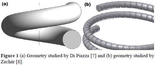
The majority of cases researched by Zachar in this study are laminar flow with a Reynolds number of between 100 and 7000. Perhaps only in cases of higher flow was it possible for some turbulence to be produced, so that the momentum equation was based on the Navier-Stokes equations. Zachar also reports having employed SIMPLE to solve the continuum and momentum equations [8].

With all of this in mind, we set out in our study to validate numerical models of heat exchangers developed with the commercial pack ANSYS®. We selected and configured the turbulence models of standard k-ε and k-ω to compare its results with those obtained in experimental and numerical studies of heat exchangers enhanced with double passive technique.

In the end, we verify the increase in heat transfer associated with the change in the geometry of the exchanger. Moreover, we discuss the importance of selecting the appropriate temperature for the evaluation of temperature-dependent fluid properties, after presenting their influence on the results.

2. Methods

CFD has been used for the following studies on various types of heat exchangers: maldistribution of the flow of fluids, dirtiness or incrustations, fall in pressure, and thermal analysis in the design and optimization phase. To perform the simulations, different turbulence models have been adopted which are generally available for commercial purposes (standard, realizable, RNG, RSM, and SST) relative to the numerical models of pressure-velocity coupling (such as SIMPLE, SIMPLEC, PISO, etc). The quality of the solutions obtained from the simulations has been within the acceptable range, demonstrating that CFD is an effective tool for predicting the behavior and performance of a broad range of heat exchangers [9].

In the course of this research, the SIMPLEC algorithm was used for solving the thermo-fluid models that involve the use of the energy equation and equations that characterize the behavior of the flow field. This is where the Navier-Stokes equations model for laminar flow and the turbulence models k-ε, realizable k-ε, and k-o appear. Below, the SIMPLEC algorithm and turbulence models are described; the boundary conditions used to describe the exchangers are characterized, and finally the applied model of comparison is presented

2.1 SIMPLE algorithm

A simple time-saving approach for the solution of the problems of conjugate heat transfer with fluid mechanics is to use a single computational domain containing the solid and fluid regions, such as Semi-Implicit Method for Pressure-Linked Equations (SIMPLE) algorithms, namely: SIMPLE, SIMPLER, SIMPLEC, etc. [10]. In CFD, the SIMPLE algorithm is a numerical method used to solve the Navier-Stokes equations. Developed by Professor Brian Spalding and his student Suhas Patankar at Imperial College London in the early 70s, it is now the basis of many commercial packages. A modified variant, the SIMPLER algorithm (SIMPLE Revised), was developed by Patankar in 1979, while another variant, SIMPLEC\' (SIMPLE-Consistent) was designed by Van Doormal and Raithby [11]. The algorithm is iterative. The basic steps for upgrading the solution are as follows [12]:

1. Selection of boundary conditions.

2. Calculation of velocity and pressure gradients.

3. Solution of the momentum equation to calculate the average velocity field.

4. Calculation of uncorrected mass flows in the boundaries. 5. Solution of the pressure correction equation to produce corrected pressure values in the grid cells.

5. Updating the pressure field.

6. Updating pressure correction at the boundaries.

7. Correction of mass flows at the boundaries.

8. Correction of velocities in the grid cells.

9. Updating the density due to pressure changes.

2.2. Turbulence model

Turbulent flow is the type of viscous flow that is applied to most industrial-use heat exchangers. Nonetheless, its analytical treatment is not as well developed as the laminar flow [13]. The main turbulence models are grouped into three families. The first are the Reynolds-averaged Navier-Stokes (RANS) equations obtained by time-averaging equations of motion over a coordinate in which the mean flow does not vary. The second is Large Eddy Simulation (LES) which solves large-scale flow motion while approximating small-scale motions. The third is Direct Numerical Simulation (DNS), in which Navier-Stokes equations are solved for all scales of turbulent flow motion, increasing accuracy as well as the time required for the calculation [14].

Models from the RANS family allow steady state solutions and model all types of turbulence without resolving the largest eddies. They are the only simulation modeling approach in steady-state for turbulent flows, and therefore are the most widely-used method for industrial flows. This is true even if the motion of eddies in a turbulent flow is inherently unstable and three-dimensional, and even if the flow is stationary in an average sense. Simulations of steady state are preferred for many engineering applications because their easiness, quick simulation time, simplified post-processing, and because, in many cases, there is only interest in time-averaged values [15].

Most models from the RANS family use k (turbulent kinetic energy) and e (rate of turbulent energy dissipation) as a basis for simulation. The difference between each of the family's models is in how approximations for unknown correlations are taken. There are three methods to address the problem of turbulence in the RANS family: Reynolds Stress Models (RSM), Algebraic Stress Models (ASM), and Eddy Viscosity Models (EVM). In the latter method, there are models of zero, one, or two equations, referring to the number of additional EDs necessary for closing the turbulent problem.

The standard k-ε model comes from the work of Chou in 1945, Davidov in 1961, and Harlow in 1968, but it was not until 1972 that Jones and Launder perfected it [16]. It was in 1974 that the model's locking coefficients were adjusted, bringing it to the form that most researchers use today, and that is the base for nearly all CFD software [17]. This model is semiempirical and in its derivation the flow is assumed to be fully turbulent, and the effects of molecular viscosity are assumed to be negligible.

Another version of the model was called "realizable" by Shih in 1995. It satisfies certain limitations in the term of normal stresses since the Boussinesq approximation, and the definition of turbulent viscosity are combined to obtain an expression for normal Reynolds stress in incompressible flow. In this way, a new definition is introduced wherein some coefficients that had been considered constant are no longer constant [18].

The k-ω model, developed by Wilcox in 1998, was the first full turbulence model. It is seen as full because besides having an equation for modeling k; it has a parameter c for the rate of dissipation of energy in units of volume and time [19]

2.3. Geometries

All analyses were carried out using different tools offered by the ANSYS® package. Nonetheless, the geometries were developed with the Siemens SolidEdge® and imported in the generic format .igs to the DesignModeler® module, where they were repaired to facilitate their discretization. The meshes were made in the Meshing® module, and simulations were configured with the CFD modules CFX® and Fluent® to corroborate the results between them.

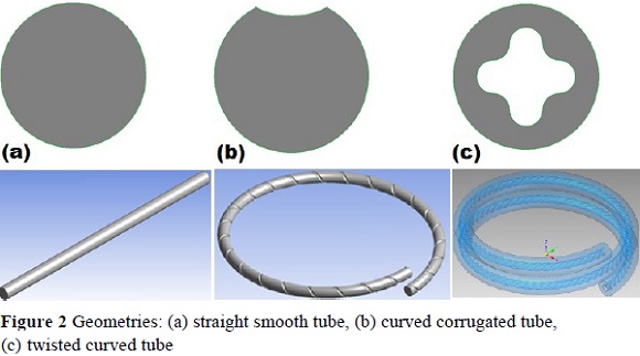
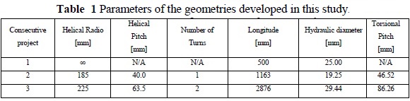
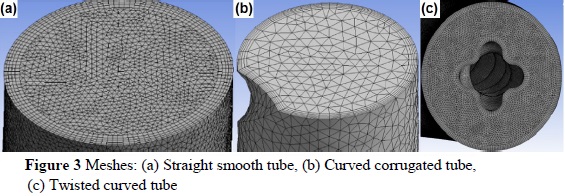
This study has three simulation projects that differ in their geometries. Swept protrusion was used for developing volumes of internal flow control and defining the profile of the cross sections required in establishing the paths. For the development of the volume of external control in the third study, the above procedure was followed to determine the geometry that served as a tool for implementing a Boolean subtraction volume operation. To develop the second and third geometry we used the torque tool that builds the sweep operation by twisting the profile of the cross-section around the path curve. The geometries are presented in Figure 2. In Table 2, the geometrical parameters of all three studies are reported.

The geometries were imported into DesignModeler® with a file extension .igs. It is a vector graphic file format 2D/3D based on the Initial Graphic Exchange Specification (IGES), for the cleaning and repairing of typical problems such as small edges, splintered faces, holes, seams and sharp angles. This allows the models prepared for the analysis to be used appropriately [20]

2.4. Meshes

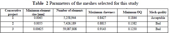
Discretization was carried out in the Meshing® module following the methodology proposed by the software developers. With the automatic method we selectively and automatically combined tetrahedra, prisms, and hexahedra, and selected the physical CFD in the global control selector. The densification of the mesh was subsequently performed by changing the minimum size, respecting the 100:1 ratio between the maximum face size and minimum face size, and the 2:1 ratio between the maximum element size and the maximum face size.

The minimum size allowed gradually decreased below the initial default option, generating an increase in the number of elements. Then we proceeded to the specification of local controls, where inflation was employed to produce prism layers applied to faces to increase the mesh resolution and resolve the viscous boundary layer in CFD. Next, we reviewed the quality parameters as recommended, which indicate ideal skewness and Orthogonal Quality (OQ) values, trying to maintain the minimum OQ > 0.1, or the maximum skewness <0.95. However, these values may be different depending on the physics and the location of the cell [21].

For the geometries associated with the projects, a densification and mesh independence study was performed with different comparison criteria. In the end, the best meshes for executing simulation projects were selected (Figure 3). The principle metrics are reported in Table 2.

2.5. . Boundary Conditions

One of the challenges in CFD is how to deal with the thin sublayer near the wall, where the viscous effects become important. In heat transfer flows, an accurate resolution of this layer is crucial because the majority of the temperature change is produced through it. The safest way is to use a fine mesh and a model with a low Reynolds number, which is computationally expensive, particularly in 3D. The slow convergence can also be a problem as a result of high aspect ratio cells. The traditional industrial solution has been to use wall functions [22].

In the solid contours of the geometry studied, the classic law-of-the-wall is used by establishing that the average velocity of a turbulent flow at a given point is proportional to the logarithm of the distance from that point to the wall, or the limit of the fluid region. This law-of-the-wall was first published by Theodore von Karman in 1930 [23].

The law-of-the-wall describes the relationship between the velocity profile and shear stress in the turbulent boundary layers. Near the wall, on the inside of the boundary layer there is a universal velocity profile. This universal behavior forms the basis for modeling near the wall in RANS. The modeling approach with wall functions is applied to cases where high resolution is unavailable near the wall. There, functions fill the space between the wall and the logarithmic law region where the first cell centroid is found.

The importance of y⁺ insensitive wall treatment is that in practice, maintain a prescribed y+ value in the cells adjacent to the wall in the entire domain of industrial cases is a challenge. Additionally, maintaining a y⁺ value such that the first node of the mesh is in the log-law region when wall functions are used can be especially problematic when the mesh is refined. Therefore, y⁺ insensitive wall treatments are a critical requirement for the use of RANS models in CFD, applied to industry [15].

One of the advantages of the k - ω model is the near-wall treatment for low Reynolds calculations because it does not involve the complex nonlinear functions required for the k - ε model. This model usually requires a near-wall resolution of y⁺ < 0.2, while the k - oi requires a minimum of y⁺ < 2. Achieving these values in industrial flows can not be guaranteed in most applications. Therefore, a new near-wall treatment was developed for the k - ω model, allowing for a smooth change from one form of low Reynolds to a wall function formulation. The automatic wall treatment allows for consistent refining of coarse mesh and insensitive y⁺, even though for highly accurate simulations, such as heat transfer predictions, a mesh with y⁺ around 1 is recommended [24].

For our study, we used constant boundary conditions, Dirichlet condition, and constant wall temperature (Table 3). It is clear that the hot wall of the last project is internal while the external wall was configured as adiabatic. The constant thermal boundary conditions of temperature and flow are different from the conditions found in reality, which may affect the Nusselt number. The change in velocity and the properties or temperature of the fluid on one side of the exchanger can affect heat transfer and fluid flow on the other. The increase in velocity increases the transfer rate, affecting the average temperature of the other substance.

If the viscosity decreases, the average pressure drop does too and depending on the pump used, there could be an increase in flow velocity. Therefore, it is important to research and understand the effects of the properties, and how the flow rates and geometry can affect the heat transfer characteristics in industrial application [21] The variation in temperature along the flowpath affects their properties and causes changes in the convective heat transfer coefficient. Density, viscosity, thermal conductivity, and specific heat are temperature-sensitive properties [25].

In the three projects, the temperature of inlet fluid (liquid water) is constant at 20°C. In the fluid configuration, the liquid water is defined from the database of the CFD module. The properties were modified to an average temperature value of 21.4°C in the first project and 23.7°C in the second, although they were left constant for all velocities evaluated. In contrast, in the third project the ideal average temperature was assessed at each velocity and the range varied between 23.7 and 33.8°C for the highest and lowest speeds.

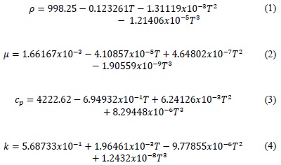
These values were estimated iteratively after running the first simulations and evaluating the results. The property values was predicted with polynomials presented by Zachar [8] and Jayakumar [2]:

Where:

T: Average temperature of the medium [°C]

p: Density [kg/m3]

µ: Dynamic viscosity [Pa.s]

c_p: Specific heat [J/kgK]

k: Thermal conductivity [W/mK]

The projects led to the building of Nusselt number vs Reynolds number or Dean number data clouds, which characterize the flow and depend on the average flow velocity. The assigned values for each project are shown in Table 3.

The geometric characteristics and the boundary conditions were chosen based on experimental studies that were used for comparison in the first two projects and as a result of independence research in the last project.

3. Results

In the first project, we worked initially with constant properties at a temperature of 25°C without knowing what temperature the fluid would reach in the exchanger. Figure 4(a) shows the comparison between Sieder and Petukhov's predictions of experimental correlations [26] against the theoretical predictions of the simulation with Fluent® and with CFX®, using the standard fc - e model. Figure 4(b) shows the same comparison, but now the fc - oi model is used; note the influence on the selection of the model when comparing Figure 4 (a) and Figure 4(b).

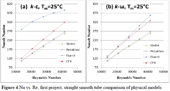
After evaluating the results and making an estimate of the outlet temperature, we proceeded to recalculate the average temperature at which to evaluate the properties of the fluid. Figure 5(a) shows the results of the comparison against theoretical results reached with the fc - oi model, but now with an average temperature of 22°C. After a sequence of iterations, an average temperature value of 21.4°C was reached. Figure 5(b) shows the results of this last sequence of simulations, affected by the mean temperature value in which the thermo-dependent properties are evaluated. In the end, the match between the CFX® results and Petukhov's predictions was achieved.

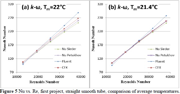
The Fluent® results were approaching this during the process but never reached the same setting as those of CFX®. This is due to differences in the default configuration and having worked with a single average temperature characteristic for all the Reynolds evaluated when the average temperature value depends on velocity.

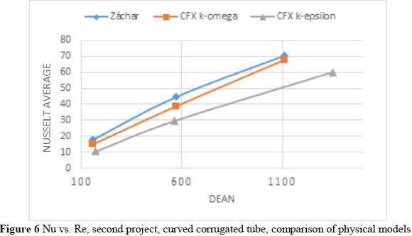
For the second project, we took advantage of the experience gained in the first. We only worked with the CFX® module, and established an average temperature value iteratively, reaching a great fit. The comparison between the numerical predictions correlation proposed by Zachar [8] against the numerical predictions of this study with CFX® using the standard k-ε model and k-ω model is presented in Figure 6.

In this project, the results of the mesh independence study are reported with both models. In Figure 7(a) we can see the errors relating to the finer mesh in the study with standard k - ε, and in Figure 7(b) with k - ω. Note the lack of definition convergence in Figure 7(a) compared to Figure 7(b). It shows that for the geometric and boundary conditions of this study, the results can be improved with the refinement of the mesh using the k - ω model.

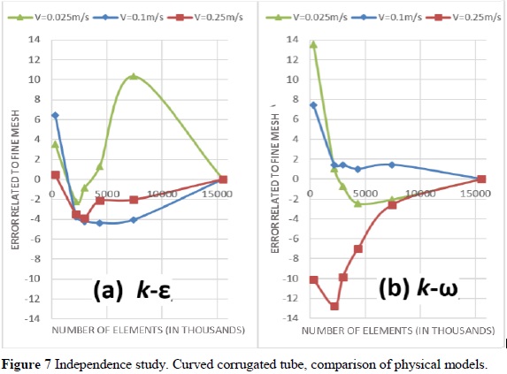
The comparative results of Figure 7 correspond to the studies of the mesh selected for its combination of economy and precision. For each velocity studied, the increase in mesh density is verified to approach the result obtained with the finer mesh increasingly. However, notice that in study advanced with the k - ε model for average velocity, a divergence appeared that could be due to a configuration error.

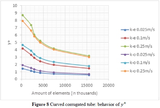
In this simulation project, particular attention was paid to the behavior of y⁺. One can see in Figure 8 a comparison of the models, of which it is independent. Note the impact of mesh refinement on the magnitude of y⁺, which decreases so that the first node gets closer and closer to the wall. The lower ranges correspond with slower flow velocities. All the velocities in this second project are relatively small, corresponding to more industrial applications like laminar flow regimes. For fully turbulent flows, more similar to industrial application, higher y⁺ values are obtained.

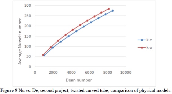
For the last project, we harvested the experience gained in the first two. We worked solely with the CFX® module and iteratively established an average temperature value, but independently from velocity. The average temperature property for each of the 10 configured velocities was carried out in this way. Figure 9 shows the comparison of the numerical predictions using CFX® with the standard k-ε model and the k-ω model. One can appreciate the great fit reached after the mesh independence study, showing as well certain independence of the model, which was to be expected.

The small differences are due to differences in the meshes after selecting the physical CFD model, since Meshing® offers options for Fluent® and CFX® that generate similar but not identical meshes, and another series of small default configuration differences for some model parameters, algorithms, and criteria.

It should be noted that for this project the independence of the results of the exchanger length was studied. For this geometry, there are no correlations, experimental results, nor numbers available in the scientific literature for validation. Figure 10 reports the incidence of mesh refinement in the magnitude of y⁺.

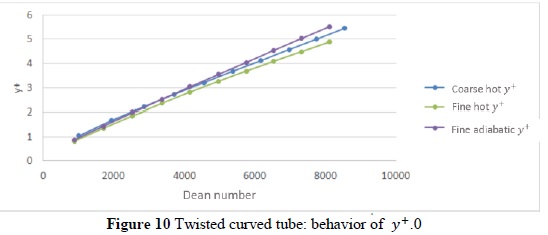
Note again that upon increasing the turbulence, the first note moves away from the wall, making the capture of the boundary layer phenomenon increasingly difficult. Since this project always evaluated averaged properties for the entire device, this does not noticeably affect the results.

Note also that when comparing the coarse mesh y + with the fine mesh, in the case of the hot wall (interior), the slight approach to the first node to the wall can be seen, consistent in the entire domain of Dean evaluated

4. Conclusions

This project allowed us to validate the theoretical results that can be achieved with commercial CFD tools by showing their approximation to experimental results. But one must keep in mind that the theoretical simulation results with commercial packages are influenced by the model selected, its configuration, meshing quality, the selection and configuration of the algorithm, and other parameters such as the convergence criteria or different geometric conditions unique to each system under study, such as heat exchanger ength.

The independence of all these factors should be evaluated before using the numerical results in making design decisions - it is often necessary to use experimental results for such validation. The RANS models are the only simulation modeling approach for turbulent flows in steady state, and in many cases there is only interest in the time-averaged values. There, increased accuracy in the development of models in the family does not represent a significant change in the averaged results in the steady state. However, if computing time increases, still the continuity of this research project will continue to use the k - ω model and CFX® model.

Nonetheless, it remains necessary to continue evaluating other models and studying the independence of various parameters. It is hoped that this report will be useful for fluid researchers who use simulation methodology in their work

Acknowledgments

This article is derived from the P13134 research project "Development of correlations of heat transfer and pressure drops in twisted tube heat exchangers - Stage II: Validation of numerically developed correlations," conducted by the research group Advanced Materials and Energy (MATyER), at the Instituto Tecnológico Metropolitano (ITM), whom we thank for their patronage and recognition.

References

[1] V. Kumar, S. Saini, M. Sharma y K. Nigam, «Pressure drop and heat transfer study in tube-in-tube helical heat exchanger,» Chemical Engineering Science, vol. 61, n° 13, pp. 4403-4416, 2006.         [ Links ]

[2] J. Jayakumar, S. M. Mahajani, J. Mandal, P. K. Vijayan y R. Bhoi, «Experimental and CFD estimation of heat transfer in helically coiled heat exchangers,» chemical engineering research and design, vol. 86, n° 3, pp. 221-232, 2008.         [ Links ]

[3] J. Jayakumar, S. M. Mahajani, J. Mandal, K. N. Iyer y P. K. Vijayan, «Thermal hydraulic characteristics of air-water two-phase flows in helical pipes,» chemical engineering research and design, vol. 88, n° 4, pp. 501-512, 2010.         [ Links ]

[4] R. Kharat, N. Bhardwaj y R. Jha, «Development of heat transfer coefficient correlation for concentric helical coil heat exchanger,» International Journal of Thermal Sciences, vol. 48, n° 12, pp. 2300-2308, 2009.         [ Links ]

[5] I. Conté y X. F. Peng, «Numerical and experimental investigations of heat transfer performance of rectangular coil heat exchangers,» Applied Thermal Engineering, vol. 29, n° 8-9, pp. 1799-1808, 2009.         [ Links ]

[6] H. P. Neopane, «Sediment Erosion in Hydro Turbines,» Norwegian University of Science and Technology, Trondheim/Norway, 2010.         [ Links ]

[7] I. Di Piazza y M. Ciofalo, «Numerical prediction of turbulent flow and heat transfer in helically coiled pipes,» International Journal of Thermal Sciences, vol. 49, n° 4, pp. 653-663, 2010.         [ Links ]

[8] A. Zachár, «Analysis of coiled-tube heat exchangers to improve heat transfer rate with spirally corrugated wall,» International Journal of Heat and Mass Transfer, vol. 53, pp. 3928-3939, 2010.         [ Links ]

[9] M. Aslam Bhutta, N. Nayat, M. Bashir, A. Rais Khan, K. Naveed Ahmad y S. Khan, «CFD applications in various heat exchangers design: A review,» Applied Thermal engineering, vol. 32, n° 1, pp. 1-12, 2012.         [ Links ]

[10] X. Cheng y P. Han, «A note on the solution of conjugate heat transfer problems using SIMPLE-like algorithms,» International Journal of Heat and Fluid Flow, vol. 21, n° 4, pp. 463-467, 2000.         [ Links ]

[11] D. S. Jang, R. Jetli y S. Acharya, «Comparison of the PISO, SIMPLER, and SIMPLEC algorithms for the treatment of the pressure-velocity coupling in steady flow problems,» Numerical heat transfer, vol. 10, n° 3, pp. 209-228, 1986.         [ Links ]

[12] P. J. Coelho y M. Carvalho, «Application of a domain decomposition technique to the mathematical modelling of a utility boiler,» International journal for numerical methods in engnieering, vol. 36, n° 20, pp. 3401-3419, 1993.         [ Links ]

[13] J. R. Welty, C. E. Wicks y R. E. Wilson, Fundamentos de Transferencia de Momento, Calor y Masa, 2 ed., México: Limusa Wiley, 2006.         [ Links ]

[14] A. Piña Ortiz, Estudio numérico y experimental de la transferencia de calor en una cavidad vertical cerrada alargada, Sonora, México: Universidad de Sonora, 2011.         [ Links ]

[15] G. Eggenspieler, «Turbulence Modeling,» 14 May 2012. [En línea]. Available: http://www.ansys.com/staticassets/ANSYS/Conference/Confidence/San%20Jose/Downloads/turbulence-summary-4.pdf. [Último acceso: 2014]         [ Links ].

[16] B. E. Launder y D. B. Spalding, «The numerical computation of turbulent flows,» Computer Methods in Applied Mechanics and Engineering, vol. 3, n° 2, pp. 269-289, march 1974.         [ Links ]

[17] J. R. Toro Gómez, Dinámica de Fluidos con introducción a la Teoría de la Turbulencia, Bogotá, Colombia: Ediciones Uniandes -Universidad de los Andes, 2006.         [ Links ]

[18] T. H. Shih, W. W. Liou, A. Shabbir, Z. Yang y J. Zhu, «A new k-ε eddy viscosity model for high Reynolds number turbulent flows,» Computers & Fluids, vol. 24, n° 3, pp. 227-238, 1995.         [ Links ]

[19] N. A. Rodriguez Muñoz, Estudio numérico de la transferencia de calor con flujo turbulento en una cavidad alargada con ventilación, Sonora, México: Universidad de Sonora, 2011.         [ Links ]

[20] M. J. Pirani, M. Da Silva y N. Manzanares, «Estudio comparativo entre el modelo de turbulencia K-e y el modelo algebraico del tensonr de reynolds,» Informacion Tecnologica, vol. 10, n° 4, pp. 253-259, 1999.         [ Links ]

[21] ANSYS, «ANSYS CFX-Solver Theory Guide,» Ansys Inc., Canonsburg, 2009.         [ Links ]

[22] ANSYS, «ANSYS DesignModeler,» [En línea]. Available: http://www.ansys.com/Products/Work flow+Technology/ANSYS+ Workbench+Platform/ANSYS+DesignModeler. [Último acceso: 2014]         [ Links ].

[23] ANSYS, Inc. , «ANSYS Meshing,» ANSYS, Inc. , 2014. [En línea]. Available: http://www.ansys.com/Products/Workflow+Technology/ANSYS+Workbench+Platform/ANSYS+Meshing. [Último acceso: 2014]         [ Links ].

[24] T. J. Craft, «Wall Function,» December 2011. [En línea]. Available: http://cfd.mace.manchester.ac.uk/twiki/pub/Main/TimCraftNotesAll_Access/advtm-wallfns.pdf.         [ Links ]

[25] T. Rennie y V. G. S. Raghavan, «Effect of fluid thermal properties on the heat transfer characteristics in a double-pipe helical heat exchanger,» International Journal of Thermal Sciences, vol. 45, n° 12, pp. 1158-1165, 2006.         [ Links ]

[26] T. Bergman, A. Lavine, F. Incropera y D. DeWith, Introduction to Heat Transfer, 6th Edition, Wiley, 2011.         [ Links ]