


 English (pdf)
 Article in xml format
 Article references
 Send this article by e-mail
 Cited by SciELO
  Cited by Google
  Similars in
SciELO
Similars in
SciELO  Similars in Google
 Permalink
1. Introduction
With the objective/aim of contributing to the establishment for a vertical global reference system that unifies altimetric data from Ssouth American countries, initiative led by Sigas Workgroup III, arises the necessity to evaluate, identify and diagnose the state of each component for the vertical reference system at a local level. The components are: Leveling network, Densification of gravimetric network, Geoidal model and Generation of geopotential numbers.
Geodetic leveling as a basic component for the adjustment of vertical networks, must have a standard methodology for the treatment of leveling data, with respect to the correction of height differences obtained in the field and their corresponding geodetic adjust; given that the development of the local vertical reference system is one of the responsibilities of the Inner Workgroup in Geodesy at (IGAC).
The procedure for geodetic leveling has not presented considerable modifications in a long time, as to methodology of field surveying is referred, since geodetic equipment hasn't evolved significantly. However, data processing at the office has presented certain computing difficulties, due to the inexistence of a general method in the pertinent procedures for captured data. Hence, the determination of corrections and leveling data adjustment are proposed and explained step by step, and the correlative least-squares method, the structure of condition equations and the contents of the matrixes are presented.
With the result of geodetic adjustment the degree of precision and accuracy of field surveyed points is determined, such that one can determine the order of the geodetic network at which the points can be integrated, besides identify for which project types the national framework can be used, according to their specifications and/or accuracy. The article is structured in the following way: first we approach the procurement of the digital leveling field surveyed data; next, the determination and computation of corrections according to technical specs of the levels used. Then, we tackle the computation of adjustment with the correlative least-squares method for the corrected height differences; and last, we present and analyze the results obtained.
2. Materials and Measurement Methods
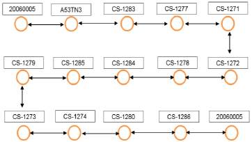
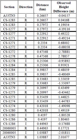
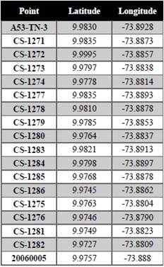
The field measurement method is realized through routines where the raw data is obtained with the digital levels. Leveling is executed in double path sections, round travels, where the length of the sections can be established between 0.8 and 1.5 kilometers, with first order closing errors [1]. The data provided by the Geographic Institute Agustín Codazzi belong to a leveling path of the urban area in Bosconia, Colombia, and follow the schematic presented in Figure 1. The field information is presented in Table 1.
3. Corrections to leveling data
Considering that no field observation is exempt of measurement errors, either generated by natural conditions or by observer's flaws, among other systematic errors that can affect the process, we have identified such aspects that lead to an inaccurate value in the leveling data. Six factors have been identified that can have an influence in the measurement true value [2]:
Calibration scale in the level staff.
Temperature of the level staff.
Atmospheric refraction.
Inexistence of horizontality in the leveling instrument line.
Effects of Moon and Sun on the Earth's equipotential surfaces.
Non-parallelism of equipotential surfaces Here, we briefly describe each one of the corrections.
Here, we briefly describe each one of the corrections.
3.1. Correction to the Level Staff scale
The objective of this correction is to verify if the length of the level staff scale is within the guidelines of the standard longitudinal norm. In general, such correction is given by the manufacturer though a calibration, however, if this information is not available, the correction process is resumed in a comparison of the length measurements in the level staff scale with respect to a standard meter. The correction of the level staff scale is calculated with equation 1 [3], and is added with the resulting algebraic sign to the observed height difference:

where:
C r = Correction to the level staff scale, in millimeters.
D = Observed height difference for the section, in meters.
e = Excess of average length of the level staff pair, in mm/m.
3.2 Temperature Correction
The temperature correction of the level staff is applied to the height difference between reference points using the mean of observed temperatures at the beginning and end of a section. This is calculated with equation 2 [3] and is added with the resulting algebraic sign of the observed height difference in the field:

Where:
C t = Temperature correction of the level staff.
tm = Average temperature observed in the level staff.
ts = Standard temperature in the level staff.
D = Observed height difference between reference points.
CE = Mean thermal expansion coefficient per unit length, per temperature degree in the level staff pair.
With respect to these variables, it should be noted that:
The average temperature is determined by the average between the temperature measurements at the beginning and the end of the section (section is the interval between materialized adjacent points).
The units of D, tm and ts must coincide with the units of CE [2].
3.3 Refraction Correction
The atmospheric refraction phenomenon is presented when "the ray incoming from the target point does not follow a rectilinear trajectory but suffers successive refractions when travelling through a variable density atmosphere" [4]. While the refraction phenomenon varies depending on the conditions in the data acquisition instant, in case one can assume that conditions such as temperature and atmospheric pressure are homogenous along the section, this correction can be omitted.
To minimize the effect of refraction, equation 3 is suggested. Is noted that this is a reconsideration of the simplified version of the model developed by Professor T.J. Kukkamäki, of the Finnish Geodetic Institute [5][6].

Where:
R = Refraction correction for the section, in millimeters.
S = Section length, in meters.
δ = Temperature difference between temperatures at 1,3 m and 0,3m above the ground, in degrees Celsius.
D = Height differences, in cm.
3.4 Collimation Correction
This correction comes to be the simplest of all, given that it refers to the coincidence in measurements in back-view and forward-view for a point must be exact; when the comparison between these two views differs from zero, this value is known as collimation error. This correction is added with the resulting algebraic sign of the observed height difference with equation 4 [2].

Where:
C c = Level collimation correction, in millimeters.
e = Collimation error, in radians x 1,000 or in mm/m.
SDS = Accumulated differences of the longitudinal views for the section, in meters (forward-view and back-view).
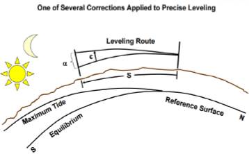
3.5 Astronomical Correction
"Astronomical correction is applied to consider the effect of tide acceleration due to the Earth's equipotential surfaces on which the Sun and Moon are located" [2]. The main characteristic of this correction is that is suggested for leveling networks of great density, due that its incidence in leveling data for local networks is insignificant (this affirmation is linked to the context of the desired precision in the leveling network being developed).
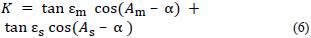
The calculation is determined by equations 5 and 6 [7]:

where:
C α = Astronomic correction.
S = Section length.
εm= Deflection due to the Moon.
εs = Deflection due to the Sun.
A s = Azimut for the Sun.
A m= Azimut for the Moon.
α = Azimuth for the section.
The 0.7 is a constant based on Earth's elasticity [8].
3.6 Orthometric Correction
Considering that each height difference taken in the field is subject to a level surface related to topography and not to a constant physical surface, orthometric correction compensates the lack of parallelism of the geometric level surfaces, taking into account the range of latitude in the leveling line, direction of the line, latitude differences and average line height [9]. Equation 7 calculates approximate orthometric correction (based on normal gravity) for the observed height difference in a section [2].
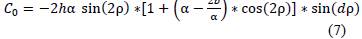
where:
C 0 = Orthometric correction.
h = Average he.ight for the section.
α = 0.002644
b = 0.000007.
p = Average latitudes for the section.
dp = latitude difference between initial and final points of the section (dp is positive when the final point of the section is located northwards of the initial point; this considering the direction of the leveling).
In the case of having real values for the gravity in each leveling point (not normal gravity), the recently proposed orthometric correction must be replaced by the formulation of geopotential numbers, which will determine a more accurate orthometric bound.
As to the orthometric bound is referred, is estimated that it can vary from very few millimeters to some decimeters with respect to the geometric bound, since its value depend not only of the ground topography, but also of the material lying underground [10]. After correcting the field leveling values, the next step is to adjust the leveling network in aim to compensate the closing error.
3.7 Practical Case
The corrections previously mentioned are all necessary in the leveling process. However, according to the type of equipment and the field survey methodology managed by the Geographical Institute Agustín Codazzi, one must consider the following annotations:
Correction of the level staff scale must not be conducted in height differences, since the staff's material is Invar and satisfy the standard calibration scale guaranteed by the manufacturer [1].
Refraction correction is programmed in the digital level, which automatically computes the correction as follows [11]:

where:
r k = Refraction coefficient of the equipment.
E = Distance of leveling change.
R = Earth's radius (6380000 m).
Collimation correction or collimation error is corrected in field by the appointed commission, employing the Förstner method, as specified in the procedure manual [1].
Astronomical correction must not be conducted in height differences, since the leveling circuit is too small, meaning that the survey is local, and its application is not required.
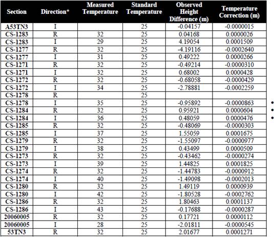
Temperature correction must be performed for each of the obtained height differences in the field. For example, for the first height difference, the value of thermal expansion in the Invar level staffs employed at IGAC is 0.000009 [12], the standard temperature of the staff is 25°C [13]. Then, the temperature correction is obtained as follows:
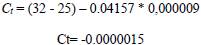
From this calculation the temperature correction is obtained for each height difference, as presented on Table 2. As an example for the height difference that corresponds to the section between A53-TN-3 and 20060005, with the following data:
Table 2 Temperature Correction.
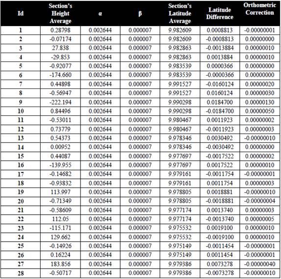
• Orthometric correction must be performed for each height difference obtained in the field. Initial data available in table 3 and table 4.
Latitude of 20060005 is 9.9757, latitude of A53-TN-3 is 9.9830, with a latitude average of 9.9794. The average height of the section is equal to 1.83856 m, a is equal to 0.002644 and ß is equal to 0.000007, latitude difference is 0.0073278. Then, the orthometric correction is equal to:
C o = -2*(1.83856*0.002644)*(sin (2*9.9794))*
[1+(0.002644-((2*0.000007) / 0.002644)*
(cos (2*9.9794))]*(sin (0.0073278))
Therefore,
C o =0.0000004.
From this calculation, orthometric correction is obtained as shown on Table 5.
4. Network adjustment
For the elimination of closing errors according to the corresponding mathematical requirements, the principle of least-squares is applied. This principle is based on searching that the sum of the squared residues from a set of observations is minimal through the most probable value (MPV) for a quantity obtained through repeated observations of equal weight [14]. To find this value that minimizes the sum of the squared residues, first one should identify:
The values of the known vertices or bounds (in case the circuit is closed; is not necessary).
The unknowns or height differences (dh) to be adjusted.
The bounds to be corrected as product of the height differences adjustment.
The distances between sections.
The direction of the circuit or leveling line.
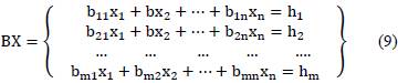
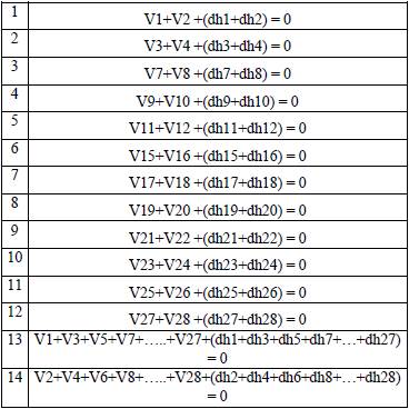
As a basis, we should provide a main system of equations or general equations. These equations will define the standard or general relationships, will depend on the context of the network and they will be the basis of comparison and a-posteriori correction of observation errors.
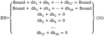
Now, for the practical case we add the height differences to a bound, which makes the final value equal to that of the considered bound, both in the forward and backward direction. Additionally, height differences in forward and backward directions for a section should add up to zero.
For the practical case one should also provide a system of observation equations that will have the unknowns as a function of observations, with the following characteristics:
The number of observations should be greater or equal than the number of unknowns.
Equations should hold no mathematical relation between them (should be linearly independent).
All measured magnitudes should be expressed through the selected equations.
The number of observation equations is given by n - k:
n = Number of measured observations.
k = number of unknowns.
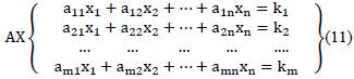
The coefficients in the condition equations (Table 6) will define the first matrix, Matrix A, which is a m x n matrix (m = number of equations, n = number of observations). Roman numerals point to the employed equations.
The values given as a solution of the AX equation systems will produce a series of remainders when replaced in the BX equation system. These values will conform the second matrix, Matrix W, which is a m x 1 matrix (m = number of equations).

According to the proposed condition equations, matrices A and W are:
In geodetic leveling, given the measurements context, the weights will be a function of the leveling lines extension. "Weights of the leveling lines are inversely proportional to their lengths, and given that the length is proportional to the number of station setups, weights are also inversely proportional to the number of station setups" [15], which is why we will consider as leveling weights the inverse relation with respect to length.

Weight values will define the third matrix, Matrix P, a diagonal matrix of n x n (n = number of observations) with elements P i .
Theoretically "the sum of the product of the weights multiplied by their respective remainders squared has to be minimized, that is the condition that should be imposed in the adjustment of weighted least squares" [12] [15]. This, represented in an equation is:

In order to minimize the function and for the equations to have a unique solution, a system of Gauss normal equations is defined. This system is defined as the partial derivatives of the remainders summation with respect to each unknown and are established as equal to zero (16).
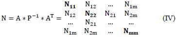
To specify matrix notation of the Gauss normal equation system, we will design the transpose matrix of Matrix A as AT, and inverse matrix of matrix P as P-1. The fourth matrix is matrix N, square matrix and symmetric with respect to the main quadratic diagonal that contains the coefficients of the normal equations. This matrix is of size m x m (m = number of equations).
The next step is the computation of the correlative factors, auxiliary factors that will be introduced in the condition equations, looking to find the minimum for the sum of the squared remainders using the LaGrange method. This methodology is known as compensation by correlative method. The values of these factors shall define the fifth matrix, matrix K, of size m x 1 (m = number of equations).
Last, the minimum quadratic solution of the observations X is obtained from solving the correlative equation system, and from these equalities one can find the desired corrections Vi. Obtaining such corrections Vi over the observed values allows to eliminate the closing errors W in the equations.
The relationship between the correlative values and the observations matrix, with their respective weights is given by the sixth matrix, matrix V, of size n x 1 (n = number of observations).
So, the compensated values for the measured observations are computed using equation 15:

where:
X = Adjusted or compensated value.
X_i = Observation value.
V_i = Correction.
5. Errors
With the purpose of evaluating the degree of functionality for the cited adjustment, the different errors are defined below.
5.1 Observation Error
The definition starts from the concept of variance. Considering that the square root of the variance of an observation represents its standard deviation or quadratic mean error, equation 16 is cited, since it's the equation that better defines said quadratic mean error [15].
In order to express the quadratic mean error as a function of the compensations, based in the equation P_1 W_1+P_2 W_2+⋯+P_n W_n= ΣP_iW_i, one can reach the following inequality [15]:
Following an intermediate mathematical development is concluded that "the mean error for an isolated observation in a set of m observation relations with a lower number of unknowns n is obtained through the following expression" (16).
The sum of the squared compensations within the radical can be rewritten as follows:

Now, considering that the compensations made are weighted, the quadratic mean error of the observation is defined as:
With the purpose of weighting the mean error for each of the observations, we use the following equation
Here mi is the mean error of the original observations.
5.2 Adjusted Value Error
Given the intervention of field observations for the computation of adjusted or compensated values, these results are also characterized by a mean error. The errors in the compensated bounds are in function of the initial measurement errors, which is known as propagation of error.
For the case of altimetric leveling, a propagation of error is generated, since the initial field measurement error is intrinsic in the compensated bound error. Given that the function that relates compensated height with field observation (height difference) is linear, the propagation of error is linear in a circuit or leveling line (Figure 3).

Here:
H_B=Bound for B.
H_A=Bound for A.
dh_AB=Height difference from A to B.
6. Precision of determined quantities
Though adjustment, the unknowns are determined indirectly, i.e., they are determined from indirect observations related to the expected unknowns through linear functions, such as observation equations; then, the standard deviation for the unit weight is expressed as [15]:
Here m is the number of observations, n is the number of unknowns. Thus, m - n are the degrees of freedom.
The precision of height differences is determined from the covariance matrix formed from the coefficients of the unknowns in the observation equations.
This is used to calculate the standard deviations of the adjusted values that are indirectly determined and are functions of observed values; the covariance matrix is equal to the inverse matrix of the normal equation coefficient matrix multiplied by the unit variation

The calculated standard deviation Si, for any given unknown, having been computed from an observation equation system, can be expressed as
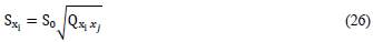
Where Qij is the diagonal element (row i, column j) from the covariance matrix [15].
7. Results and discussion
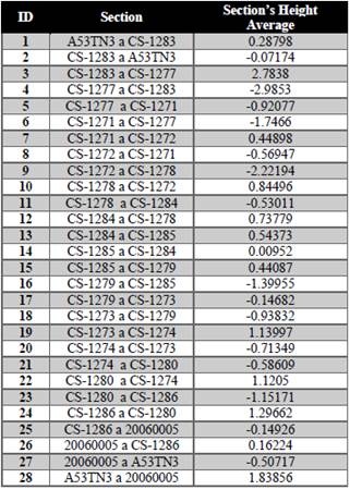
The proportionality of corrections inference in height differences is presented in figure 4. Orthometric corrections were less considerable in all height differences, with respect to the temperature correction, whence is concluded that the leveling zone can present a constant gravity model.
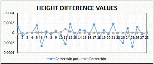
However, as previously mentioned, the way of precisely stating this affirmation is through geopotential numbers. Thereby, the respective corrections for the circuit data obtained in field by the Geographic Institute Agustín Codazzi are summarized in Table 7.
Regarding the least-squares adjustment, the calculated mean squared error was 0.05478 centimeters. The observation equations were selected with the criteria of conditioning the adjustment towards a bound closing, both in forward and backward directions.
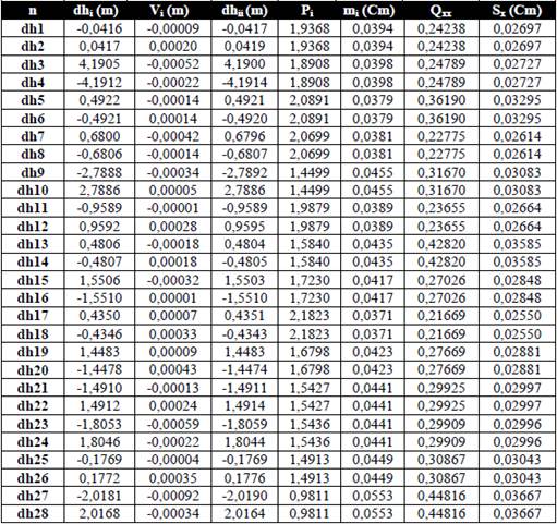
Also, the remaining equations are related taking as a rule that both the forward and backward direction height differences must be equal, thus their sum should be equal to zero. Obtained results are presented in Table 8, where:
n = Height difference.
dh= Height difference Initial value (without adjustment corrections).
Vi (m) = Obtained corrections.
dhii (m) = Corrected height difference value.
Pi = Weight for each height difference.
mi (m) = Mean error for original observations. See equation 21.
Qxx = Correlation factor.
Sx (m) = Mean error for adjusted observations. See equation 25.
8. Conclusions
Corrections made to the obtained height differences in field did not exceed 0.1 mm on average, but in some sections the corrections come to 0.03 centimeters. Although the corrections do not modify considerable the height differences, these should not be disregarded, since geodetic leveling is based on high accuracy precisions, whereby a variation comparable to a centimeter is considerable for height differences that usually don't exceed 1 meter.
Additionally, depending on the extension or location of the survey, physical factors documented in the corrections (temperature, height, latitude, etc.) may vary in greater extent, hence the corrections can be greater.
Accuracy of adjustment for the leveling circuit is reflected in the quadratic mean error equivalent to 0.06 centimeters. This error represents an accuracy confidence around half millimeter, which is remarkable considering the accuracy required in geodesy.
The reason that led to the high accuracy of the adjustment was, at first an optimal definition of the initial observation equations in which the basic principles for the practical leveling case were considered.
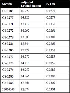
The precision range for the obtained adjusted heights varies between 0.0255 and 0.0358 centimeters, which represents a standard deviation around half a millimeter, assuring highly precise leveled height values.
Obtaining high precision values for each measurement enables the use of geodetic information separately, i.e. after the adjustment each height difference can be used in different projects depending their requirement of precision and accuracy; this provides different companies and entities more accurate and independent altimetric values.
For the Geographic institute Agustín Codazzi the determination of a local vertical reference system has become a very important aim, due to the desire of contributing to the establishment of the global vertical reference system. The computation of geopotential numbers and normal heights is a first approximation to the obtention of such systems, and since adjusted geometric height differences are one of the main inputs for said computation, this article supplies the need of standardizing leveling data treatment in the office.

