


 Inglês (pdf)
 Artigo em XML
 Referências do artigo
 Enviar este artigo por email
 Citado por SciELO
  Citado por Google
  Similares em
SciELO
Similares em
SciELO  Similares em Google
 Permalink
1. Introduction
The United Nations estimates that by 2030 two-thirds of the world's population will live in cities (United Nations, 2019). This poses great challenges to the increasingly populated cities, and to face them the Smart City concept arises as a type of urban development that uses the potential of technology and innovation to promote sustainable development and, in short, improve the quality of life of the citizens of these cities (Founoun & Hayar, 2018).
One of the goals of a Smart City is to give all individuals access to better mobility and transportation solutions, including public transportation (Vernier et al., 2016). However, to promote its use, it is important to improve access to it, which implies strengthening the weakest links: first-mile transport (from the starting point to a public transport station) and last-mile transport (from a bus station to the destination) (Chong et al., 2011; Vernier et al., 2016).
Autonomous vehicles can offer a solution to first and last mile transportation (Boston Consulting Group, 2016), and their integration with public transportation can provide a sustainable door-to-door solution (Shen et al., 2018). This has motivated the academic community, the automotive industry and technology companies to investigate ways to give vehicles greater autonomy (Hartmannsgruber et al., 2019). Special interest is being placed on the achieving of precise and reliable localization in urban areas (Brenner, 2009; Payá et al., 2017; Qu et al., 2018), which implies acquiring information on any instant of position and orientation with respect to a reference frame or map using information from a sensory system (Thrun et al., 2006).
The most widely used system to obtain the position of a vehicle is the GNSS (Global Navigation Satellite System) (Kuutti et al., 2018). However, in urban areas, there may be interruptions in the reception of the signal and multiple paths (Cui & Ge, 2003; Kos et al., 2010), which makes it less reliable. This has motivated the use of relative motion information through odometry and inertial navigation systems (INS), but these bring error accumulation with it over time, generating a high level of uncertainty with regards to localization (Soheilian et al., 2016).
To improve the robustness, reliability and precision in the localization of vehicles, information from their environment is implemented using sensors such as cameras and / or 2D / 3D LiDAR (Light Detection and Ranging) and techniques for the construction of maps and data association (Kuutti et al., 2018). The cameras provide abundant information, but their performance declines when the lighting is not adequate. On the other hand, a 3D LiDAR is less sensitive to changes in lighting, its field of view is 360°, and it provides distance information. However, storing and processing point clouds can be very expensive from a computational standpoint. An alternative is to only use information from representative elements of the environment or landmarks, thus making the storage and processing more efficient (Vivacqua et al., 2018).
Natural elements present in urban roads (e.g. trees) (Brenner, 2010) or artificial elements (e.g. traffic signal poles, traffic lights or electricity poles) have been used as landmarks (Li et al., 2021; Schlichting & Brenner, 2014; Weng et al., 2018), and these can be easily extracted due to some physical characteristic (geometry or appearance), and are stable in the long term (Brenner, 2010; Schaefer et al., 2019). Table 1 shows a summary of the most significant works that have used infrastructure elements detected by laser or LiDAR as landmarks for localization.
Table 1 Summary of localization methods that use detection of infrastructure elements.
| Article | Sensors | Landmarks | Localization method |
|---|---|---|---|
| (Brenner, 2010) | Four laser scanners. | Traffic signs, traffic lights and trees. | Pattern matching filter based on least squares. |
| (Schlichting & Brenner, 2014) | LiDAR. | Pole-like objects and building facades. | Local feature patterns. |
| (Hata et al., 2014) | LiDAR 3D. | Road curbs. | Monte Carlo. |
| (Hata & Wolf, 2014) | LiDAR 3D. | Road curbs and road marking. | Monte Carlo. |
| (Wang et al., 2017) | LiDAR 3D. | Curbs. | EKF. |
| (Weng et al., 2018) | LiDAR 3D. | Pole-like features. | Particle filter. |
| (Schaefer et al., 2019) | LiDAR 3D. | Pole-like features. | Particle filter. |
| (Lu et al., 2020) | LiDAR 3D. | Pole-like features. | Non-linear optimization. |
| (Li et al., 2021) | LiDAR 3D | Pole-like features. | Monte Carlo. |
Pole-like objects (trees, power poles, traffic lights, etc.), have been used to implement localization systems in urban environments since they are frequently found, their geometry is well defined and due to their height, they are not totally occluded by other objects. In (Brenner, 2010), they are used to build a geo-referenced map combining information from GNSS, INS and LiDAR. A disadvantage of this type of proposal is that the localization fails when the density of landmarks is low since the data association, is found to be ambiguous. For this reason, in Schlichting and Brenner (2014), other landmarks are added to the map which are composed of cylindrical objects, in this case planes (building facades), and an association technique called feature patterns, which describes the spatial relationship between the landmarks on the map, making the localization more robust.
In Weng et al. (2018), a map is built by detecting and geo-referencing pole-like objects (trees, lighting poles, etc.) which are to be used in a real-time localization system in congested urban areas. These type of objects are also used in Schaefer et al. (2019), to implement a long-term localization system in urban areas that have been tested for 15 months. In (Lu et al., 2020), this class of elements are also used to build a global map based on small local maps according to a grouping algorithm of detected objects. In the same way, Li et al. (2021), uses pole-like objects to implement a localization system that ranges from mapping to map matching, using a new algorithm for feature extraction that is more stable.
Other elements present on the roads have also been used as landmarks. In Hata et al. (2014), a 3D LiDAR is used to build a map based on the detection of road curbs, but this method presents considerable errors in the localization. To improve this, in Hata and Wolf (2014), lines and road markings are added to the map. In Wang et al. (2017), the road curbs are also used to build a map by merging information from a 3D LiDAR and a GPS, and the localization is carried out using the ICP (Iterative Closest Point) algorithm.
This paper presents a localization system for autonomous vehicles in outdoor parking lots (first and last mile environment) that uses a map based on geo-referenced landmarks (road marking poles with reflective tape). To estimate the position of the vehicle, an Extended Kalman Filter (EKF), fed with odometry information, and the observations of the landmarks by means of a 3D LiDAR are used. The implemented algorithm is evaluated in nine routes, which involves finding the error between the position estimated by the filter and the position of the vehicle registered by means of a GPS in RTK mode (Real Time Kinematics) as a means of establishing ground-truth. The results obtained show that this method has the potential to be used in locating autonomous vehicles in first-mile and last-mile environments, such as outdoor parking lots.
The main contribution of this work is the implementation of a localization system for autonomous vehicles in outdoor first/last mile environments, using a low-resolution map based on pole-like artificial landmarks and, for map matching, a nonlinear estimation algorithm such as the EKF.
2. Methods
2.1. Vehicle and sensors
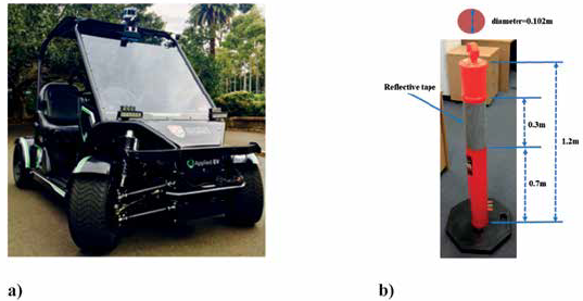
The vehicle used is shown in Figure 1 (a). This is an electric vehicle developed at the Australian Center for Field Robotics (ACFR) at the University of Sydney (Zhou et al., 2018), equipped with different types of sensors and an NVIDIA automotive computer DRIVE PX2 running ROS (Robot Operating System). A 3D LiDAR Velodyne VLP-16 mounted on the top of the vehicle was used to perceive the environment. The relative position and orientation of the vehicle are obtained using the VN-100 IMU (Inertial Measurement Unit). The global position of the vehicle is obtained by the GPS Ublox C94-M8P-D operated in RTK mode, which is used as a reference (ground-truth).
2.1. Landmarks
Orange road marking poles with reflective tape were used as landmarks, as shown in Figure 1 (b). This type of object was chosen since they are infrastructure elements that can be located in open spaces such as roads, or closed areas such as parking lots, and can be identified due to their shape and/or color. In this paper, they were detected via the reflective tape by thresholding the intensity information that the 3D LiDAR deliveres. To determine the range of intensity values corresponding to the reflective tape, the calibration process shown in figure 2 was carried out.
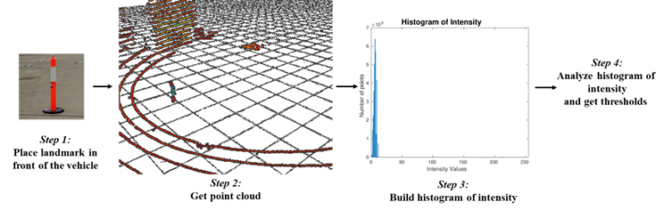
In step 1, the landmarks are located in front of the vehicle at distances between 2 m and 12 m. In step 2, the point cloud is captured for each distance. In step 3, the cumulative intensity histogram is constructed for all distances including the intensity values between 0 (poorly reflective objects) and 255 (highly reflective objects), as shown in figure 3 (a). In step 4, an intensity histogram analysis is performed using the Otsu’s Method (Otsu, 1979). This method is generally used to automatically find, in an intensity histogram, N-1 thresholds that allow the intensities to be separated into N classes, thus minimizing the variance of intra-class intensities or, equivalently, maximizing the variance of inter-class intensities.
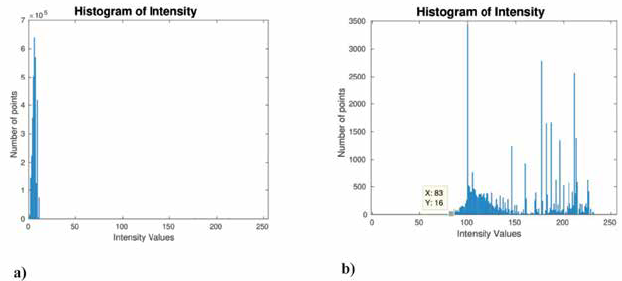
Using this method, the threshold 83 is found to make an initial separation of the histogram into two regions: the low levels (pavement and other background elements) and the high levels (elements with higher reflectivity). Figure 3 (b) shows the histogram for the intensity values between 83 and 255. It is observed that there is not a clearly defined number of classes, for this reason, thresholds for N = 2, 3, and 4 were found, as shown in table 2. Afterwards, the parameter Metric (Otsu, 1979) is evaluated, which indicates a better separability between classes the closer it is to 1. N = 4 is chosen since it was observed that an increase from 3 to 4 classes, improves the separability by about 4%.
Table 2 Thresholds and intensity intervals as a function of the number of classes (N).
| N | Thresholds | Intensity intervals | Metric |
|---|---|---|---|
| 2 | [155] | [83 155] [155 255] | 0.8377 |
| 3 | [141 190] | [83 141] [141 190] [190 255] | 0.9194 |
| 4 | [120 158 197] | [83 120] [120 158] [158 197] [197 255] | 0.9607 |
To determine which of the 4 intervals is adequate, they were tested within the point clouds thet were obtained in the 9 test runs (see section 3) and a metric was built based on the percentage of correct detections of the landmarks, since the correct landmark detection has a direct influence on the performance of the localization algorithm. Table 3 shows the results and the chosen intensity interval was [158,197], because it presented the highest percentage of correct detections.
2.2. Localization algorithm
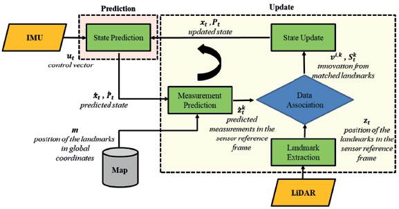
The localization of a vehicle is defined as the problem of finding at every instant of time t and with regards to a map m, the state vector x_t with its respective covariance P_t (Thrun et al., 2006). Figure 4 shows the block diagram of the implemented localization algorithm. This algorithm is based on an EKF which is a statistical filter that operates recursively in two large blocks: prediction and update. In executing the localization algorithm, four considerations are made:
i) The vehicle is moving in the X-Y plane, therefore x_t is defined according to equation 1.
Where
ii) Map
Where
iii) The state vector
In this paper, the initial position
iv) The covariance matrix
Where
As inputs, the localization algorithm receives: a map
Initially, the State Prediction block is executed which returns the predicted state vector
Subsequently, if there is a point cloud available from the 3D LiDAR, the Landmark Extraction block is executed, as shown in Figure 5. First, the point cloud is filtered by intensity-based thresholding. Second, the resulting points are grouped using the k-means algorithm according to their
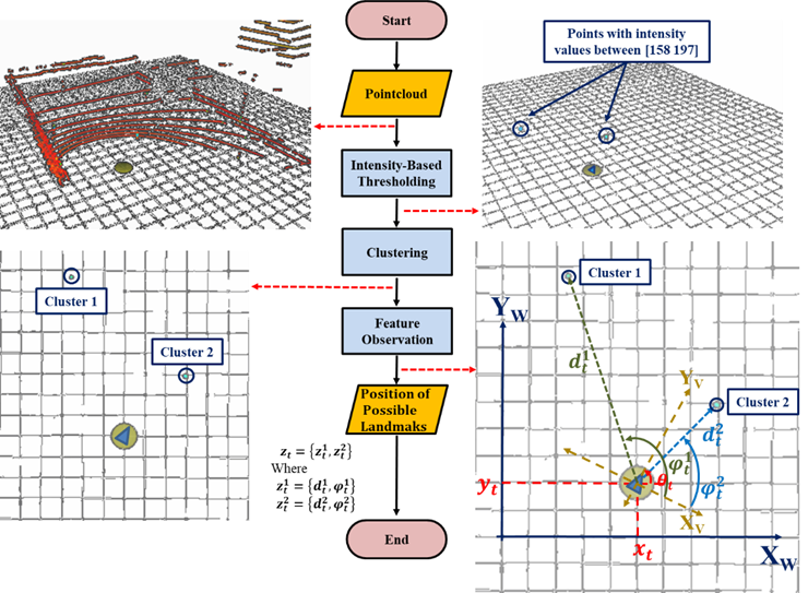
Next, the Measurement Prediction block is executed, which generates for each of the M landmarks on the map a vector
Subsequently, the Data Association block is executed using the Mahalanobis Distance (MD) (Mahalanobis, 1936), to determine for each
If a correspondence occurs, the State Update block is executed, which updates the state vector
3. Results and discussion
To evaluate the proposed location system, 8 landmarks are randomly distributed in an outdoor parking lot measuring 30 m x 40 m, as shown in figure 6 (a), and the map of the environment is constructed by manually registering the global position of these 8 landmarks using a Ublox C94-M8P-D GPS in RTK mode which delivers an accuracy of up to 2 cm, as shown in figure 6 (b).
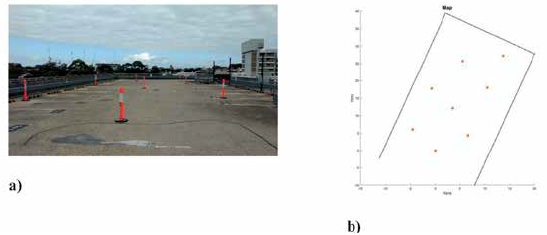
Subsequently, nine different routes are made with distances between 85 m and 360 m, and the position of the vehicle is obtained using an on board GPS Ublox C94-M8P-D operated in RTK mode. These positions are used as the ground-truth of the localization. Translational and rotational velocity are also obtained using a IMU VN-100 and point clouds with a 3D LiDAR Velodyne VLP-16.
Figure 7 shows the result of the localization for three of the nine routes using only the odometry information (prediction) as well as the output of the EKF-based localization algorithm implemented (prediction + update). In the Odometry-labelled column, it can be observed that the estimated position differs from the ground-truth for most of the path, while in the following column, the estimated position is much more precise. To make a quantitative analysis of these results, the RMSE (Root Mean Square Error) is calculated between the ground-truth and the estimated position in both X and Y, as shown in table 4.
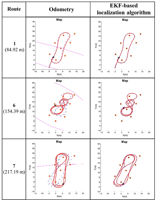
Figure 7 Result of the localization for three of the nine routes: Odometry vs EKF-based localization algorithm implementation. The blue points represent the vehicle’s ground-truth, while the red line represents the estimate position.
Tabla 4 RMSE of Odometry vs. RMSE of EKF-based localization algorithm.
| Route | Odometry | EKF-based localization algorithm | RMSE reduction | ||||||||
|---|---|---|---|---|---|---|---|---|---|---|---|
| Number | Distance (m) | RMSE X (m) | Std RMSE X (m) | RMSE Y (m) | Std RMSE Y (m) | RMSE X (m) | Std RMSE X (m) | RMSE Y (m) | Std RMSE Y (m) | X (%) | Y (%) |
| 1 | 84.92 | 0.56 | 0.45 | 0.69 | 0.68 | 0.23 | 0.23 | 0.45 | 0.45 | 58.9 | 49.4 |
| 2 | 145.39 | 0.58 | 0.42 | 0.85 | 0.64 | 0.28 | 0.28 | 0.43 | 0.43 | 51.7 | 49.4 |
| 3 | 170.39 | 1.07 | 0.31 | 0.60 | 0.56 | 0.30 | 0.30 | 0.50 | 0.50 | 71.9 | 16.6 |
| 4 | 363.13 | 0.95 | 0.50 | 0.76 | 0.71 | 0.30 | 0.30 | 0.49 | 0.49 | 68.4 | 35.5 |
| 5 | 270.37 | 1.36 | 0.71 | 0.53 | 0.47 | 0.29 | 0.29 | 0.43 | 0.43 | 78.6 | 18.8 |
| 6 | 154.39 | 2.22 | 1.86 | 1.51 | 1.11 | 0.28 | 0.28 | 0.33 | 0.33 | 87.3 | 78.1 |
| 7 | 217.19 | 2.53 | 2.50 | 1.36 | 1.34 | 0.31 | 0.31 | 0.55 | 0.55 | 87.7 | 59.5 |
| 8 | 321.32 | 2.98 | 1.89 | 1.12 | 1.09 | 0.37 | 0.37 | 0.57 | 0.57 | 87.6 | 49.1 |
| 9 | 290.12 | 1.88 | 1.42 | 1.62 | 1.61 | 0.45 | 0.45 | 0.67 | 0.67 | 76.0 | 58.6 |
It is observed that in six of the nine tours, the EKF-based algorithm implementation caused the RMSE in position X to remain less than or equal to 0.3 m, and the RMSE in position Y to remain less than 0.5 m. In addition, on all tours, the EKF-based algorithm implementation reduced the RMSE of the localization to between 50% and 90% for position X, and between 16% and 60% for position Y.
To determine the behavior of the uncertainty in the estimated position, the point-to-point standard deviation of the position in X, Y and θ was calculated for each of the routes and later correlated with the number of observed landmarks. Figure 8 shows the result for route 6. It is observed that when the position is estimated using odometry, the standard deviations grow with time, while with the EKF-based localization algorithm implementation, the standard deviations remained at a certain interval, growing gradually when only one landmark was observed, and quicly when none was detected, as seen around 10 s.
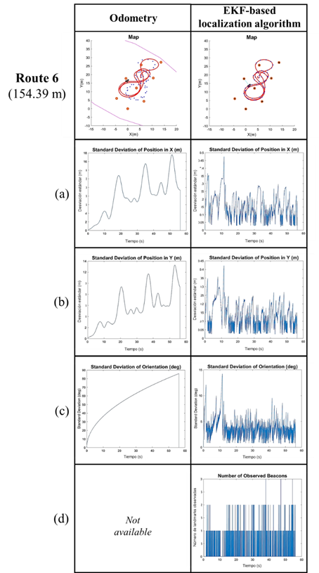
To make a qualitative analysis of the behavior of the standard deviation, the average for each of the routes was calculated and recorded in Table 5. It is observed that the average standard deviation for both the position X and Y is maintained below 0.22 m, and for orientation θ, below 5.3 °.
Tabla 5 Mean standard deviation.
| Route | Distance (m) | Mean Std. X (m) | Mean Std. Y (m) | Mean Std. θ (°) |
|---|---|---|---|---|
| 1 | 84.92 | 0.19 | 0.19 | 4.76 |
| 2 | 145.39 | 0.17 | 0.19 | 4.58 |
| 3 | 170.39 | 0.22 | 0.22 | 5.38 |
| 4 | 363.13 | 0.18 | 0.19 | 4.87 |
| 5 | 270.37 | 0.18 | 0.16 | 4.57 |
| 6 | 154.39 | 0.15 | 0.14 | 3.99 |
| 7 | 217.19 | 0.21 | 0.19 | 5.29 |
| 8 | 321.32 | 0.18 | 0.19 | 4.80 |
| 9 | 290.12 | 0.14 | 0.15 | 4.01 |
The proposed localization method is compared with the state-of-the-art method MCL method (Monte Carlo Localization) (Li et al., 2021; Schaefer et al., 2019; Weng et al., 2018), in terms of RMSE, and the results are shown in Table 6. It can be seen that with the EFK-based method, minor errors were obtained in all the routes in position X with differences between 0.10 m and 0.26 m. On the other hand, in position Y, the proposed method was overcome in four runs, but by differences less than 0.04 m. The method proposed in this paper behaves more appropiately in five runs, with differences between 0.03 m and 0.16 m.
Table 6 Comparison between the EKF-based localization method and the MCL method.
| Route | EKF-based localization algorithm | MCL algorithm | Difference MCL and EKF-based | ||||||||
|---|---|---|---|---|---|---|---|---|---|---|---|
| Number | Distance (m) | RMSE X (m) | Std RMSE X (m) | RMSE Y (m) | Std RMSE Y (m) | RMSE X (m) | Std RMSE X (m) | RMSE Y (m) | Std RMSE Y (m) | RMSE X (m) | RMSE Y (m) |
| 1 | 84.92 | 0.23 | 0.23 | 0.45 | 0.45 | 0.37 | 0.38 | 0.48 | 0.49 | 0.14 | 0.03 |
| 2 | 145.39 | 0.28 | 0.28 | 0.43 | 0.43 | 0.52 | 0.52 | 0.41 | 0.41 | 0.24 | -0.02 |
| 3 | 170.39 | 0.30 | 0.30 | 0.50 | 0.50 | 0.46 | 0.44 | 0.61 | 0.62 | 0.16 | 0.11 |
| 4 | 363.13 | 0.30 | 0.30 | 0.49 | 0.49 | 0.45 | 0.45 | 0.52 | 0.52 | 0.15 | 0.03 |
| 5 | 270.37 | 0.29 | 0.29 | 0.43 | 0.43 | 0.46 | 0.46 | 0.46 | 0.46 | 0.17 | 0.03 |
| 6 | 154.39 | 0.28 | 0.28 | 0.33 | 0.33 | 0.54 | 0.54 | 0.49 | 0.49 | 0.26 | 0.16 |
| 7 | 217.19 | 0.31 | 0.31 | 0.55 | 0.55 | 0.44 | 0.44 | 0.54 | 0.55 | 0.13 | -0.01 |
| 8 | 321.32 | 0.37 | 0.37 | 0.57 | 0.57 | 0.52 | 0.52 | 0.53 | 0.54 | 0.15 | -0.04 |
| 9 | 290.12 | 0.45 | 0.45 | 0.67 | 0.67 | 0.55 | 0.50 | 0.63 | 0.63 | 0.10 | -0.04 |
It is observed that, in general, the method proposed in this paper presents a RMSE less than or equal to the RMSE obtained by the MCL method. This may be due to the fact that the latter uses a particle filter in which the particles are dispersed a lot as time passes and no landmarks are observed, as in the experiments carried out. Therefore, this despersion can cause an increase in RMSE when calculating the state vector. However, the MCL method has the advantage of being able to deal with several localization hypothesis simultaneously, wich can be very useful when estimating the estate vector (Li et al., 2021).
4. Conclusions
In this paper, a localization system for a vehicle in outdoor environments was implemented using a map based on geo-referenced landmarks. As landmarks, road marking posts with reflective tape were used since they are elements that can be located in urban environments of the last/first mile, such as parking lots.
To estimate the position of the vehicle, an extended Kalman filter (EKF) was used, fed with odometry information and the reference points observed by means of a 3D LiDAR in nine different routes with distances between 85 m and 360 m. The results show that incorporating the information from the observations improves the estimation of the position both in X (between 50% and 90%) and in Y (between 16% and 60%). Furthermore, the mean standard deviation remains below 0.22 m for both X and Y positions, and below 5.3 ° for the θ orientation. These results indicate that this is a promising localization method for environments with previously geo-referenced landmarks that can be detected and located.
To determine the scalability of the proposed method, it is necessary to carry out tests in larger areas (for example, a university campus), building and updating a map that uses both the infrastructure landmarks and others naturally present in the given environment (power poles, traffic lights and trees) and testing the EKF-based localization method implementation under different conditions.

